Add features outside of the model for more exploration options

Shapash SmartExplainer compile method has optional parameters additional_data and additional_features_dict which allows the user to add features outside of the model for the WebApp. Those additional features can be useful for further exploration and understanding of how the model works.

This tutorial details an adequate use case.

Data from Kaggle US Accidents.

In this tutorial, the data are not loaded raw. A data preparation to facilitate the use of the tutorial has been done. You can find it here: Eurybia - Data Preparation.

import pandas as pd
from sklearn.model_selection import train_test_split
import catboost
from category_encoders import OrdinalEncoder

from shapash.data.data_loader import data_loading
df_car_accident = data_loading("us_car_accident")

Building Supervized Model

Here we are creating a binary classification model to predict the severity of an accident. We train and predict regardless of the year in which the accidents occur.

y = df_car_accident["target"]
X = df_car_accident.drop(["target", "target_multi", "year_acc", "Description"], axis=1)

features = [
    "Start_Lat",
    "Start_Lng",
    "Distance(mi)",
    "Temperature(F)",
    "Humidity(%)",
    "Visibility(mi)",
    "day_of_week_acc",
    "Nautical_Twilight",
    "season_acc",
]

features_to_encode = [
    col for col in X[features].columns if X[col].dtype not in ("float64", "int64")
]

encoder = OrdinalEncoder(cols=features_to_encode)
encoder = encoder.fit(X[features])
X_encoded = encoder.transform(X)

Xtrain, Xtest, ytrain, ytest = train_test_split(
    X_encoded, y, train_size=0.75, random_state=1
)

model = catboost.CatBoostClassifier()
model.fit(Xtrain, ytrain, verbose=False)

ypred=pd.DataFrame(model.predict(Xtest),columns=['pred'],index=Xtest.index)

Understanding my model with Shapash

Declare SmartExplainer

from shapash import SmartExplainer

features_dict = {
    "day_of_week_acc": "Day of week",
    "season_acc": "Season"
}

xpl = SmartExplainer(
    model=model,
    preprocessing=encoder, # Optional: compile step can use inverse_transform method
    features_dict=features_dict, # Optional: specifies label for features name
)

Declare additional features and compile SmartExplainer

To further understand the model we add the year and description features to our SmartExplainer compile.

additional_data = df_car_accident.loc[Xtest.index, ["year_acc", "Description"]]
additional_features_dict = {"year_acc": "Year"}

xpl.compile(
    x=Xtest,
    y_pred=ypred, # Optional: for your own prediction (by default: model.predict)
    y_target=ytest, # Optional: allows to display True Values vs Predicted Values
    additional_data=additional_data, # Optional: additional dataset of features for Webapp
    additional_features_dict=additional_features_dict, # Optional: specifies label for additional features name
)

Analyse the model with Shapash WebApp

app = xpl.run_app()

The additional features appear in the dataset with their column names in italic, starting with an underscore:

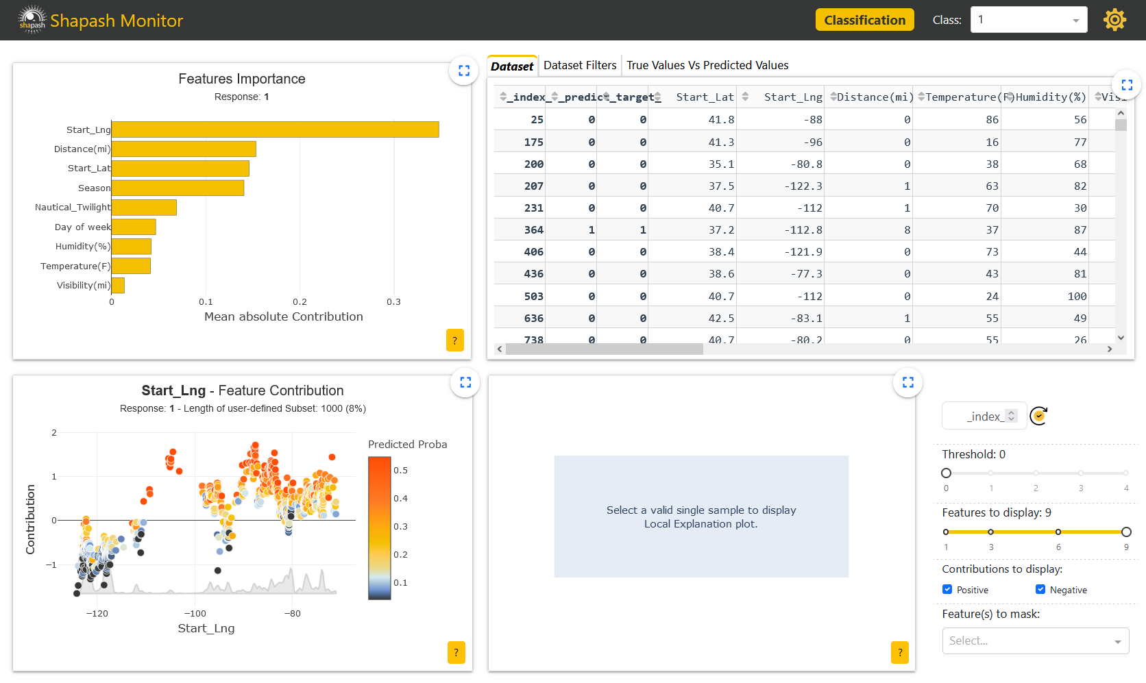
Having additional data in the WebApp allows the user to apply filters on those features to study the behavior of the model on specific subsets.

Here we can identify that the model does not work identicaly depending on the years. After applying a filter on the additional Year column to select the accidents occuring in 2019, we can see that the corresponding subset feature importances are not the same as the global ones on the Features Importance graph in the upper left corner of the screen:

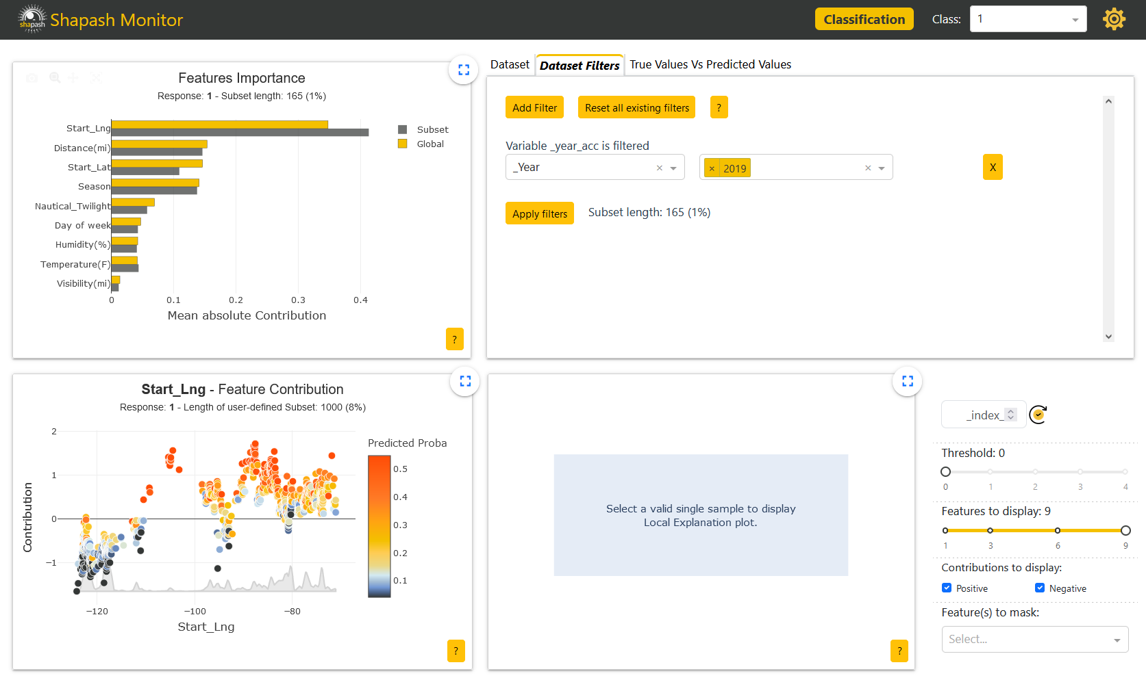
By combining our use of Shapash with Eurybia, we can see that there is indeed a significant data drift per year: Eurybia - Detect High Data Drift

Additional features can also be useful to give more details about each sample. For example, having a complete description helps us understand our sample better when exploring our model locally.

In our current case, we are now interested in understanding our wrong predictions. As one of many selection options, we can use the True Values Vs Predicted Values graph in the upper right corner of the screen to pick a specific mispredicted sample. We choose here an accident predicted as nonsevere but which is in reality:

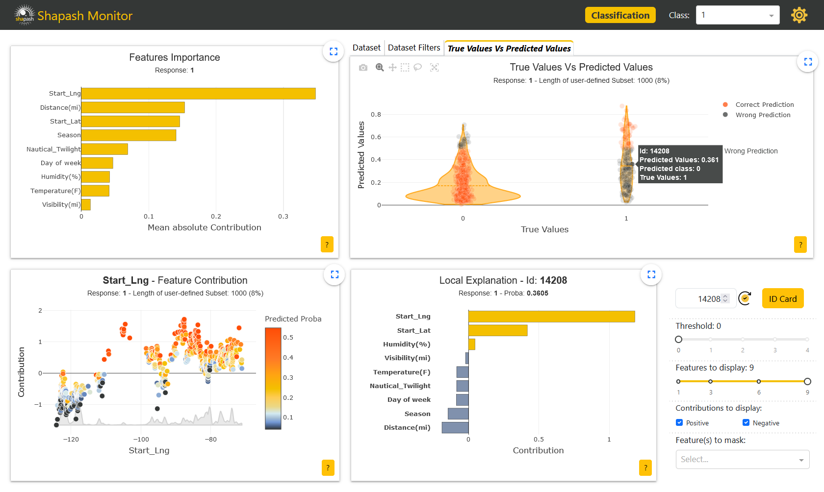
The Local Explanation graph in the rigth lower corner of the screen is now udpated with the contributions of the selected sample. It is also now possible to have a closer look at the sample thanks to the Identity Card:

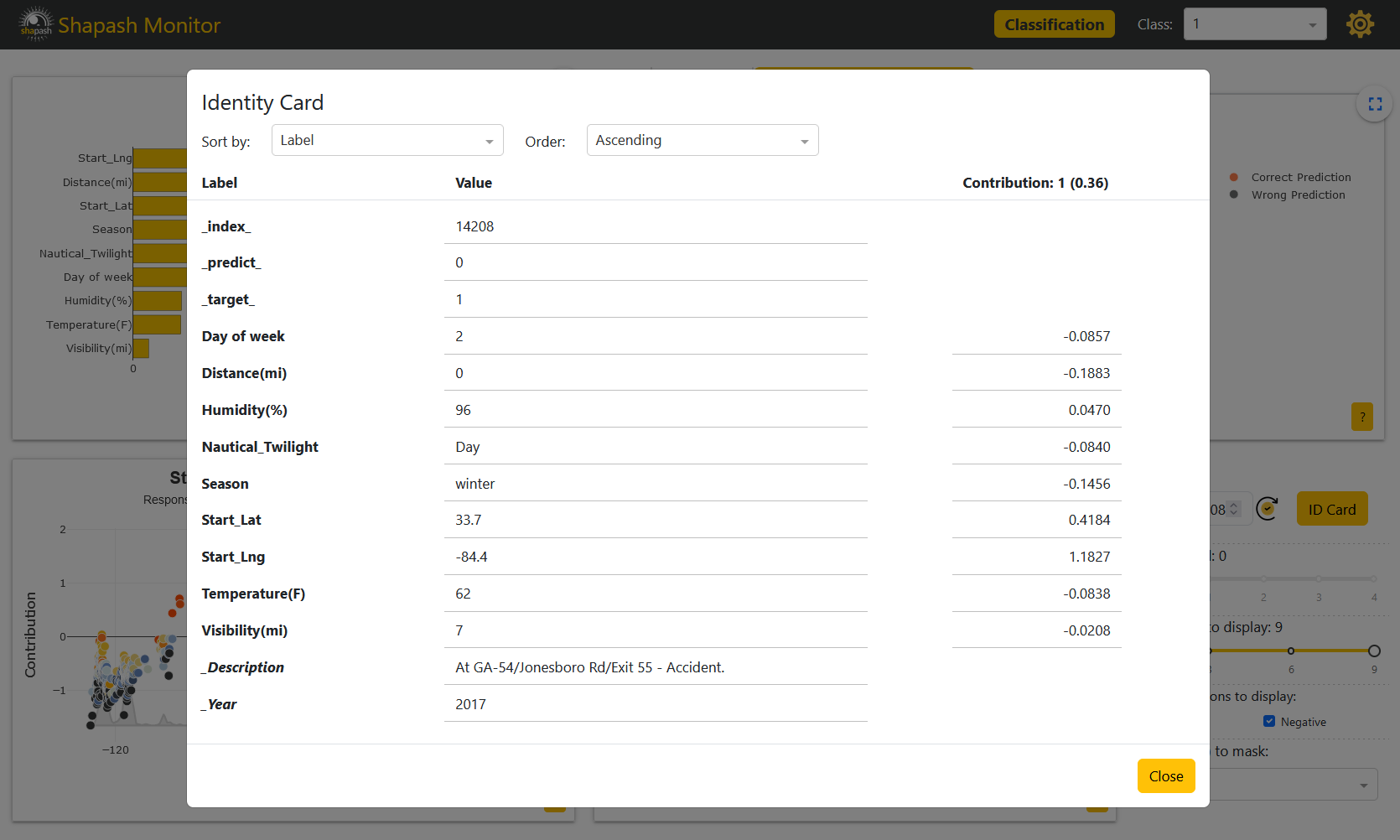
We previously gave the Description of the accidents as an additional feature. Thus the description of our selected sample appears in the Identity Card. It says that the road is closed because of the accident. This information could corroborate reality and would show that the accident is actually quite severe. Therefore, there are surely solutions to improve our model.

app.kill()