Shapash in Jupyter - Overview¶

With this tutorial you: Understand how Shapash works in Jupyter Notebook with a simple use case

Contents: - Build a Regressor - Compile Shapash SmartExplainer - Display global and local explanability - Export local summarized explainability with to_pandas method - Save Shapash object in pickle file

Data from Kaggle House Prices

[1]:

import pandas as pd
from category_encoders import OrdinalEncoder
from lightgbm import LGBMRegressor
from sklearn.model_selection import train_test_split

Building Supervized Model¶

[2]:

from shapash.data.data_loader import data_loading
house_df, house_dict = data_loading('house_prices')

[3]:

y_df=house_df['SalePrice'].to_frame()
X_df=house_df[house_df.columns.difference(['SalePrice'])]

[4]:

house_df.head()

[4]:

	MSSubClass	MSZoning	LotArea	Street	LotShape	LandContour	Utilities	LotConfig	LandSlope	Neighborhood	...	EnclosedPorch	3SsnPorch	ScreenPorch	PoolArea	MiscVal	MoSold	YrSold	SaleType	SaleCondition	SalePrice
Id
1	2-Story 1946 & Newer	Residential Low Density	8450	Paved	Regular	Near Flat/Level	All public Utilities (E,G,W,& S)	Inside lot	Gentle slope	College Creek	...	0	0	0	0	0	2	2008	Warranty Deed - Conventional	Normal Sale	208500
2	1-Story 1946 & Newer All Styles	Residential Low Density	9600	Paved	Regular	Near Flat/Level	All public Utilities (E,G,W,& S)	Frontage on 2 sides of property	Gentle slope	Veenker	...	0	0	0	0	0	5	2007	Warranty Deed - Conventional	Normal Sale	181500
3	2-Story 1946 & Newer	Residential Low Density	11250	Paved	Slightly irregular	Near Flat/Level	All public Utilities (E,G,W,& S)	Inside lot	Gentle slope	College Creek	...	0	0	0	0	0	9	2008	Warranty Deed - Conventional	Normal Sale	223500
4	2-Story 1945 & Older	Residential Low Density	9550	Paved	Slightly irregular	Near Flat/Level	All public Utilities (E,G,W,& S)	Corner lot	Gentle slope	Crawford	...	272	0	0	0	0	2	2006	Warranty Deed - Conventional	Abnormal Sale	140000
5	2-Story 1946 & Newer	Residential Low Density	14260	Paved	Slightly irregular	Near Flat/Level	All public Utilities (E,G,W,& S)	Frontage on 2 sides of property	Gentle slope	Northridge	...	0	0	0	0	0	12	2008	Warranty Deed - Conventional	Normal Sale	250000

5 rows × 73 columns

Encoding Categorical Features¶

[5]:

from category_encoders import OrdinalEncoder

categorical_features = [col for col in X_df.columns if X_df[col].dtype == 'object']

encoder = OrdinalEncoder(
    cols=categorical_features,
    handle_unknown='ignore',
    return_df=True).fit(X_df)

X_df=encoder.transform(X_df)

Train / Test Split¶

[6]:

Xtrain, Xtest, ytrain, ytest = train_test_split(X_df, y_df, train_size=0.75, random_state=1)

Model Fitting¶

[7]:

regressor = LGBMRegressor(n_estimators=200).fit(Xtrain,ytrain)

[LightGBM] [Info] Auto-choosing col-wise multi-threading, the overhead of testing was 0.001867 seconds.
You can set `force_col_wise=true` to remove the overhead.
[LightGBM] [Info] Total Bins 2986
[LightGBM] [Info] Number of data points in the train set: 1095, number of used features: 66
[LightGBM] [Info] Start training from score 182319.757078

[8]:

y_pred = pd.DataFrame(regressor.predict(Xtest),columns=['pred'],index=Xtest.index)

Understand my model with shapash¶

Declare and Compile SmartExplainer¶

[9]:

from shapash import SmartExplainer

[10]:

xpl = SmartExplainer(
    model=regressor,
    preprocessing=encoder, # Optional: compile step can use inverse_transform method
    features_dict=house_dict  # Optional parameter, dict specifies label for features name
)

[11]:

xpl.compile(x=Xtest,
 y_pred=y_pred,
 y_target=ytest, # Optional: allows to display True Values vs Predicted Values
 )

INFO: Shap explainer type - <shap.explainers._tree.TreeExplainer object at 0x7f259c8e77c0>

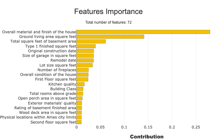
Display features importance¶

[12]:

xpl.plot.features_importance()

[12]:

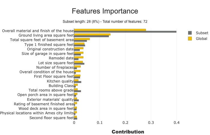
../_images/tutorials_tutorial02-Shapash-overview-in-Jupyter_19_0.png

Focus on a specific subset¶

You can use the features_importance method to compare the contribution of features of a subset to the global features importance

[13]:

subset = [ 168, 54, 995, 799, 310, 322, 1374,
          1106, 232, 645, 1170, 1229, 703, 66,
          886, 160, 191, 1183, 1037, 991, 482,
          725, 410, 59, 28, 719, 337, 36]
xpl.plot.features_importance(selection=subset)

[13]:

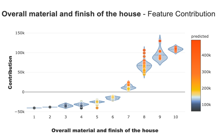
../_images/tutorials_tutorial02-Shapash-overview-in-Jupyter_21_0.png

Understand how a feature contributes¶

The contribution_plot allows to analyse how one feature affects prediction
Type of plot depends on the type of features
You can use feature name, feature label or feature number to specify which feature you want to analyze

[14]:

xpl.plot.contribution_plot("OverallQual")

[14]:

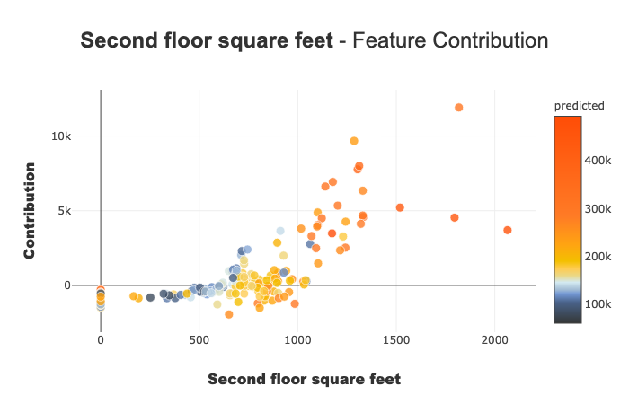
../_images/tutorials_tutorial02-Shapash-overview-in-Jupyter_23_0.png

[15]:

xpl.plot.contribution_plot("Second floor square feet")

[15]:

../_images/tutorials_tutorial02-Shapash-overview-in-Jupyter_24_0.png

Display a Summarized but Explicit local explainability¶

Filter method¶

Use the filter method to specify how to summarize local explainability There are 4 parameters to customize the summary: - max_contrib : maximum number of criteria to display - threshold : minimum value of the contribution (in absolute value) necessary to display a criterion - positive : display only positive contribution? Negative?(default None) - features_to_hide : list of features you don’t want to display

[16]:

xpl.filter(max_contrib=8,threshold=100)

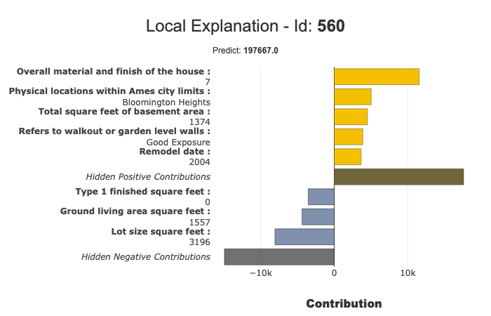
Display local plot, applying your filter¶

you can use row_num, index or query parameter to specify which prediction you want to explain

[17]:

xpl.plot.local_plot(index=560)

[17]:

../_images/tutorials_tutorial02-Shapash-overview-in-Jupyter_29_0.png

Save your Explainer & Export results¶

Export your local explanation to pandas DataFrame:¶

to_pandas method has the same parameters as the filter method

[18]:

summary_df= xpl.to_pandas(
    max_contrib=3, # Number Max of features to show in summary
    threshold=5000,
)

[19]:

summary_df.head()

[19]:

	pred	feature_1	value_1	contribution_1	feature_2	value_2	contribution_2	feature_3	value_3	contribution_3
259	211538.742157	Ground living area square feet	1792	13995.651927	Overall material and finish of the house	7	13539.441353	Total square feet of basement area	963	-5652.206854
268	178786.677257	Ground living area square feet	2192	27967.966278	Overall material and finish of the house	5	-26133.987559	Overall condition of the house	8	7799.924798
289	111985.324660	Overall material and finish of the house	5	-25571.348315	Ground living area square feet	900	-16006.763921	Total square feet of basement area	882	-5456.989325
650	73456.522515	Overall material and finish of the house	4	-34517.073676	Ground living area square feet	630	-21350.707866	Total square feet of basement area	630	-12699.371236
1234	136249.557316	Overall material and finish of the house	5	-26469.235405	Ground living area square feet	1188	-10980.550285	Condition of sale	Abnormal Sale	-5240.009373

Save your explainer in Pickle File¶

You can save the SmartExplainer Object in a pickle file to make new plots later or launch the WebApp again

[20]:

xpl.save('./xpl.pkl')