Compile faster Lime and consistency of contributions¶

You can compute your local contributions with the Lime library and summarize them with Shapash. One of the limitations of using Lime is the speed of calculation. In this tutorial, we propose 2 ways to speed up the calculations. Then, we look impacts on the contributions of these accelerated calculations.

Prerequisite: this tutorial requires lime (pip install shapash[lime]).

Contents: - Build a Binary Classifier (Random Forest) - Create Explainer using Lime - Compile Shapash SmartExplainer - Use of multiprocessing - Changing setting of the num_samples option - Comparison of computing times - Consistency of contributions

Data from Kaggle Telco customer churn

[ ]:

import warnings
warnings.filterwarnings("ignore")

[2]:

import numpy as np
import pandas as pd
from category_encoders import OrdinalEncoder
from sklearn.ensemble import RandomForestClassifier
from sklearn.model_selection import train_test_split

try:
    import lime  # noqa: F401
except ImportError as exc:
    raise ImportError("This tutorial requires 'lime'. Install it with: pip install shapash[lime]") from exc

from shapash import SmartExplainer
from shapash.explainer.consistency import Consistency

Building Supervized Model¶

Let’s start by loading a dataset and building a model that we will try to explain right after.

[3]:

from shapash.data.data_loader import data_loading

[4]:

%%time
df = data_loading('telco_customer_churn')

CPU times: user 63.1 ms, sys: 20.9 ms, total: 84 ms
Wall time: 1.71 s

[5]:

df = df.reset_index().drop('customerID', axis=1)

[6]:

df['Churn'] = df['Churn'].map({'No': 0, 'Yes': 1}).astype('int8')

[7]:

y_df = df['Churn']
X_df = df.drop('Churn', axis=1)

Encoding Categorical Features¶

[8]:

categorical_features = [col for col in X_df.columns if X_df[col].dtype == 'object']

encoder = OrdinalEncoder(
    cols=categorical_features,
    handle_unknown='ignore',
    return_df=True).fit(X_df)

X_df=encoder.transform(X_df)

Train / Test Split¶

[9]:

Xtrain, Xtest, ytrain, ytest = train_test_split(
    X_df, y_df, train_size=0.75, random_state=1
)

Model Fitting¶

[10]:

rf = RandomForestClassifier(n_estimators=100,min_samples_leaf=3)
rf.fit(Xtrain, ytrain)

[10]:

RandomForestClassifier(min_samples_leaf=3)

In a Jupyter environment, please rerun this cell to show the HTML representation or trust the notebook.
On GitHub, the HTML representation is unable to render, please try loading this page with nbviewer.org.

Compute Lime with Shapash¶

[11]:

xpl_lime = SmartExplainer(
    model=rf,
    backend='lime',
    data=Xtest[0:100],
    preprocessing=encoder,
)

[12]:

%%time
xpl_lime.compile(x=Xtest[0:100])

CPU times: user 4.58 s, sys: 39.4 ms, total: 4.62 s
Wall time: 4.62 s

The calculation times for 100 individuals are long, which is why we propose 2 ways to speed up these computation times.

These 2 ways are not yet integrated in Shapash. Fortunately, Shapash allows user to calculate his own contributions and give them as input to Shapash objects to get plots, web app, report.

Compute Lime with use of multiprocessing¶

Multiprocessing allows users to fully leverage multiple processors on a given machine. Read this documentation if you want to know more Multiprocessing

[13]:

# Function features_check Extract feature names from Lime Output to be used by shapash
def features_check(s):
    for w in list(Xtest.columns):
        if f' {w} ' in f' {s} ' :
            feat = w
    return feat

[14]:

#Training Tabular Explainer
explainer = lime.lime_tabular.LimeTabularExplainer(Xtest[0:100].values,
                                                   mode='classification',
                                                   feature_names=Xtest[0:100].columns
                                                   )

[15]:

# Definition of functions for multiprocessing-like execution in notebooks
# For this example 4 cores are used
from collections import namedtuple
from joblib import Parallel, delayed

LogEntry = namedtuple("LogEntry", ["exp", "index_row"])

contribution_list = []


def predict_proba_with_feature_names(x):
    if isinstance(x, pd.DataFrame):
        x_df = x
    else:
        x_df = pd.DataFrame(x, columns=Xtest.columns)
    return rf.predict_proba(x_df)


def foo_pool(x):
    exp = explainer.explain_instance(
        Xtest[0:100].loc[x].values,
        predict_proba_with_feature_names,
        num_features=Xtest.shape[1],
    )
    index_row = x
    return LogEntry(exp=exp, index_row=index_row)


def log_result(result):
    contribution_list.append(
        (
            result.index_row,
            {features_check(elem[0]): elem[1] for elem in result.exp.as_list()},
        )
    )


def apply_async_with_callback(n_jobs=4):
    global contribution_list
    contribution_list = []

    results = Parallel(n_jobs=n_jobs, backend="loky")(
        delayed(foo_pool)(row) for row in Xtest[0:100].index
    )

    for result in results:
        log_result(result)

Compute Lime contributions with multiprocessing

[16]:

%%time
contribution_list = []
apply_async_with_callback()

CPU times: user 1.23 s, sys: 223 ms, total: 1.45 s
Wall time: 3.33 s

By applying multiprocessing on 4 cores, the calculation time is almost divided by 4

[17]:

#transformation into a dataframe with the same column and row sorting as lime contribution dataset
contribution_multiprocessing = pd.DataFrame(pd.concat([pd.DataFrame(list(pd.DataFrame(contribution_list).iloc[:,0]),columns=['index']),
           pd.DataFrame(list(pd.DataFrame(contribution_list).iloc[:,1]))], axis=1).set_index('index'))
contribution_multiprocessing = contribution_multiprocessing[pd.DataFrame(xpl_lime.contributions[1]).columns]
contribution_multiprocessing = contribution_multiprocessing.reindex(xpl_lime.contributions[1].index)

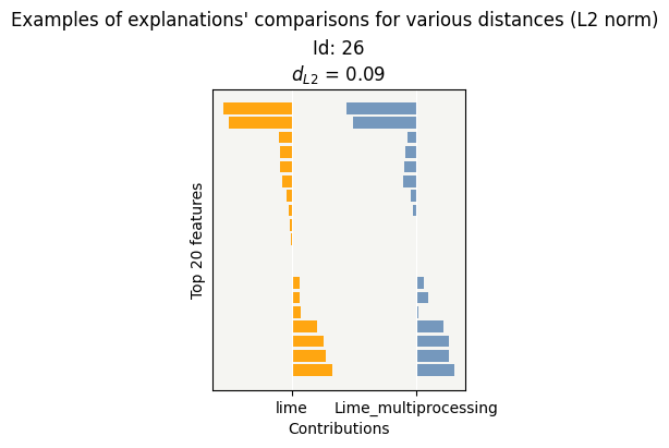
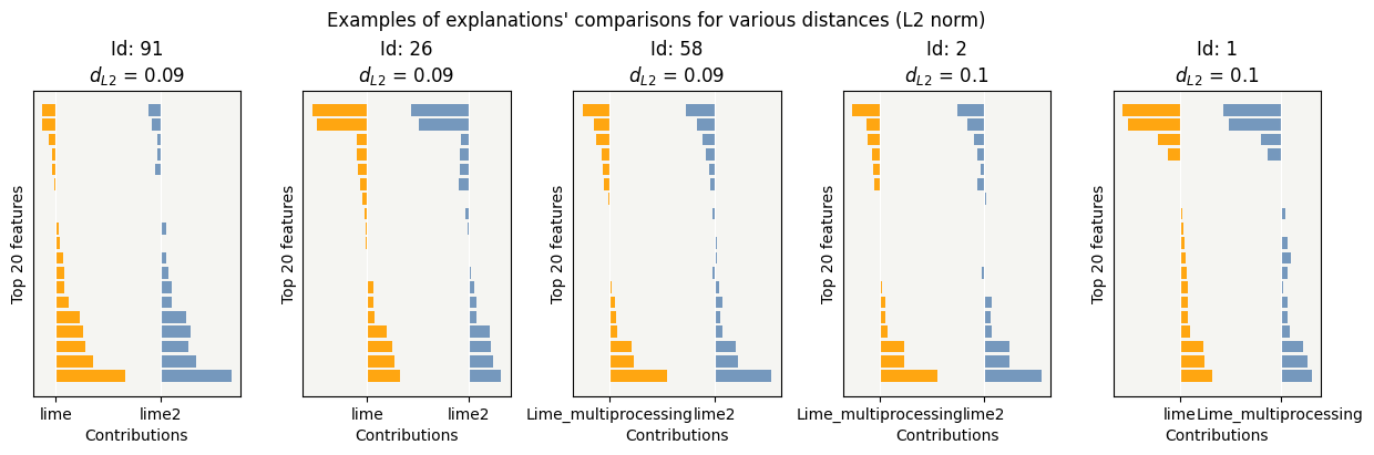
To validate that the results of the contribution calculation with multiprocessing are equivalent to the Lime calculation, we can use the object Consistency.

The Consistency metric compares methods between them and evaluates how close the explanations are from each other.

To see more details : https://github.com/MAIF/shapash/blob/master/tutorial/explainability_quality/tuto-quality01-Builing-confidence-explainability.ipynb

[18]:

#creation of the contribution dict for Consistency object
contributions = { "lime":pd.DataFrame(xpl_lime.contributions[1]).reset_index(drop=True),
                  "Lime_multiprocessing":contribution_multiprocessing.reset_index(drop=True)}

[19]:

cns = Consistency()
cns.compile(contributions=contributions)
cns.consistency_plot()

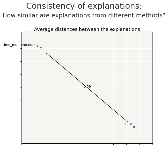
../../_images/tutorials_explainer_and_backend_tuto-expl04-Shapash-compute-Lime-faster_29_0.png

../../_images/tutorials_explainer_and_backend_tuto-expl04-Shapash-compute-Lime-faster_29_1.png

Lime works with a substitution model, which generates randomness.

The distance between the contributions by the 2 calculations is small.

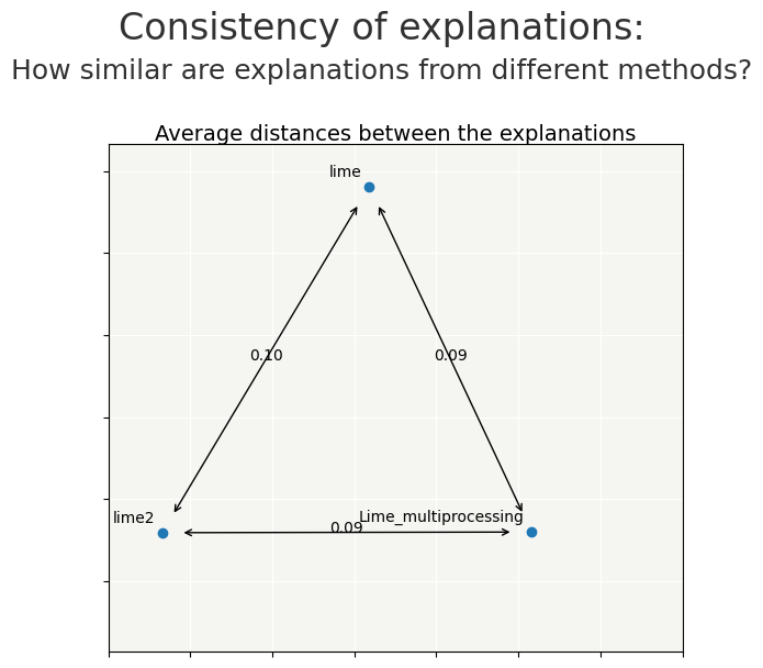
we recompile Lime to compare the differences

[20]:

xpl_lime2 = SmartExplainer(
    model=rf,
    backend='lime',
    data=Xtest[0:100],
    preprocessing=encoder,
)

[21]:

%%time
xpl_lime2.compile(x=Xtest[0:100])

CPU times: user 4.8 s, sys: 54.7 ms, total: 4.85 s
Wall time: 4.95 s

[22]:

contributions = { "lime":pd.DataFrame(xpl_lime.contributions[1]).reset_index(drop=True),
                  "Lime_multiprocessing":contribution_multiprocessing.reset_index(drop=True),
                  "lime2":pd.DataFrame(xpl_lime2.contributions[1]).reset_index(drop=True)}

[23]:

cns = Consistency()
cns.compile(contributions=contributions)
cns.consistency_plot()

../../_images/tutorials_explainer_and_backend_tuto-expl04-Shapash-compute-Lime-faster_35_0.png

../../_images/tutorials_explainer_and_backend_tuto-expl04-Shapash-compute-Lime-faster_35_1.png

Compute Lime by changing parameter num_samples¶

num_samples is the size of the neighborhood to learn the linear model. By default num_samples is 5000

if num_samples is smaller, substitution model will be less accurate, and compute will be faster

let’s test reducing num_samples to 2000 to see the time saving and the impact on the contributions

[24]:

%%time
# Compute local Lime Explanation for each row in Test Sample
contrib_2000=[]
for ind in Xtest[0:100].index:
    exp = explainer.explain_instance(
        Xtest[0:100].loc[ind].values,
        predict_proba_with_feature_names,
        num_features=Xtest[0:100].shape[1],
        num_samples=2000,
    )
    contrib_2000.append(dict([[features_check(elem[0]),elem[1]] for elem in exp.as_list()]))

CPU times: user 2.52 s, sys: 27.5 ms, total: 2.54 s
Wall time: 2.66 s

[25]:

contribution_df =pd.DataFrame(contrib_2000,index=Xtest[0:100].index)
Lime2000 = contribution_df[list(Xtest[0:100].columns)]

[26]:

contributions = { "Lime5000":pd.DataFrame(xpl_lime.contributions[1]).reset_index(drop=True),
                  "Lime2000":Lime2000.reset_index(drop=True)}

[27]:

cns = Consistency()
cns.compile(contributions=contributions)
cns.consistency_plot()

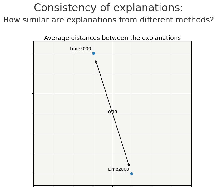
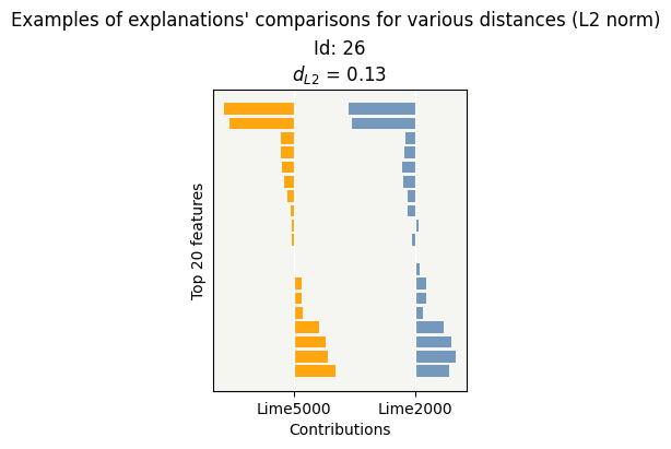
../../_images/tutorials_explainer_and_backend_tuto-expl04-Shapash-compute-Lime-faster_41_0.png

../../_images/tutorials_explainer_and_backend_tuto-expl04-Shapash-compute-Lime-faster_41_1.png

By changing the num_samples parameter from 5000 to 2000, the impact is quite small on the contributions and the time saving is close to 2.5

let’s test reducing num_samples to 1000

[28]:

%%time
# Compute local Lime Explanation for each row in Test Sample
contrib_1000=[]
for ind in Xtest[0:100].index:
    exp = explainer.explain_instance(
        Xtest[0:100].loc[ind].values,
        predict_proba_with_feature_names,
        num_features=Xtest[0:100].shape[1],
        num_samples=1000,
    )
    contrib_1000.append(dict([[features_check(elem[0]),elem[1]] for elem in exp.as_list()]))

CPU times: user 1.67 s, sys: 12.7 ms, total: 1.69 s
Wall time: 1.74 s

[29]:

contribution_df =pd.DataFrame(contrib_1000,index=Xtest[0:100].index)
Lime1000 = contribution_df[list(Xtest[0:100].columns)]

[30]:

contributions = { "Lime5000":pd.DataFrame(xpl_lime.contributions[1]).reset_index(drop=True),
                  "Lime2000":Lime2000.reset_index(drop=True),
                  "Lime1000":Lime1000.reset_index(drop=True)}

[31]:

cns = Consistency()
cns.compile(contributions=contributions)
cns.consistency_plot()

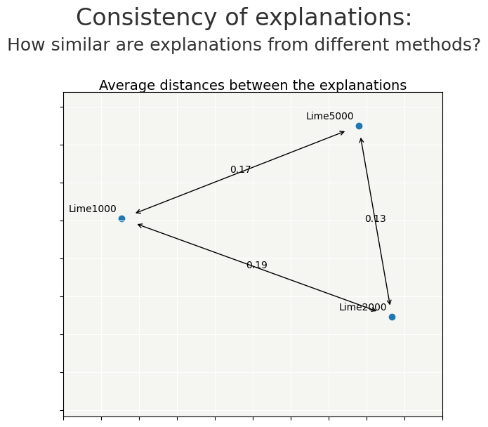
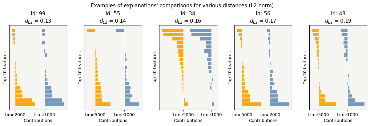
../../_images/tutorials_explainer_and_backend_tuto-expl04-Shapash-compute-Lime-faster_47_0.png

../../_images/tutorials_explainer_and_backend_tuto-expl04-Shapash-compute-Lime-faster_47_1.png

Choice of the num_samples parameter may be a compromise between quality of explicability and computation time

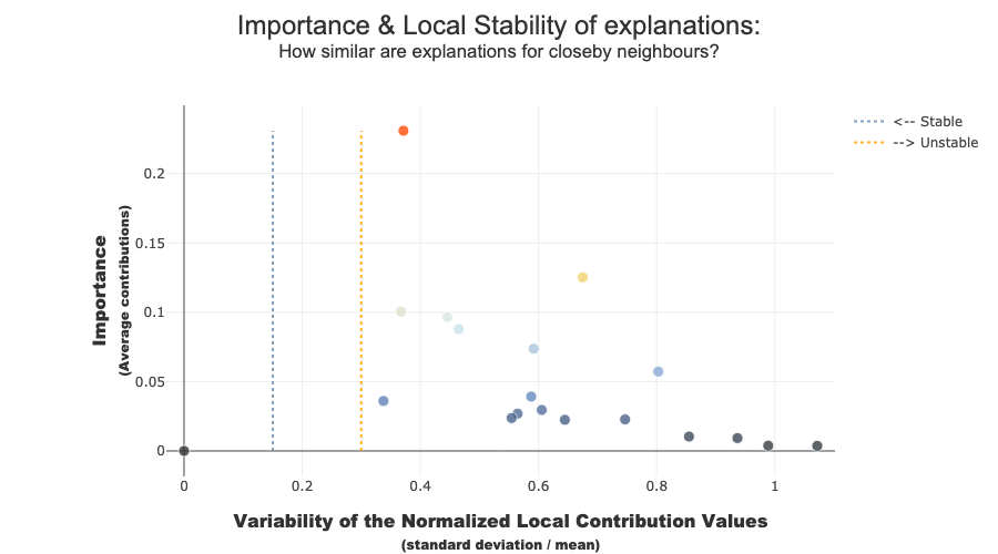
To increase confidence in the explanation, measuring their stability is important.

We define stability as follows: if instances are very similar, then one would expect the explanations to be similar as well. Therefore, locally stable explanations are an important factor that help build trust around a particular explanation.

The similarity between instances is evaluated under two criteria: (1) the instances must be close in the feature space and (2) have similar model outputs.

[32]:

xpl_lime.plot.stability_plot()

../../_images/tutorials_explainer_and_backend_tuto-expl04-Shapash-compute-Lime-faster_50_0.png

[33]:

xpl_lime2000 = SmartExplainer(
    model=rf,
    preprocessing=encoder
)

[34]:

%%time
xpl_lime2000.compile(
    contributions=Lime2000,
    x=Xtest[0:100]
)

CPU times: user 39.9 ms, sys: 5.93 ms, total: 45.8 ms
Wall time: 52.8 ms

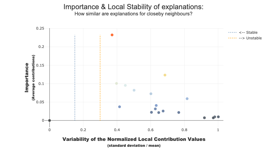
[35]:

xpl_lime2000.plot.stability_plot()

../../_images/tutorials_explainer_and_backend_tuto-expl04-Shapash-compute-Lime-faster_53_0.png

[36]:

xpl_lime1000 = SmartExplainer(
    model=rf,
    preprocessing=encoder
)

[37]:

%%time
xpl_lime1000.compile(
    contributions=Lime1000,
    x=Xtest[0:100],
)

CPU times: user 34.3 ms, sys: 3.04 ms, total: 37.3 ms
Wall time: 76.4 ms

[38]:

xpl_lime1000.plot.stability_plot()

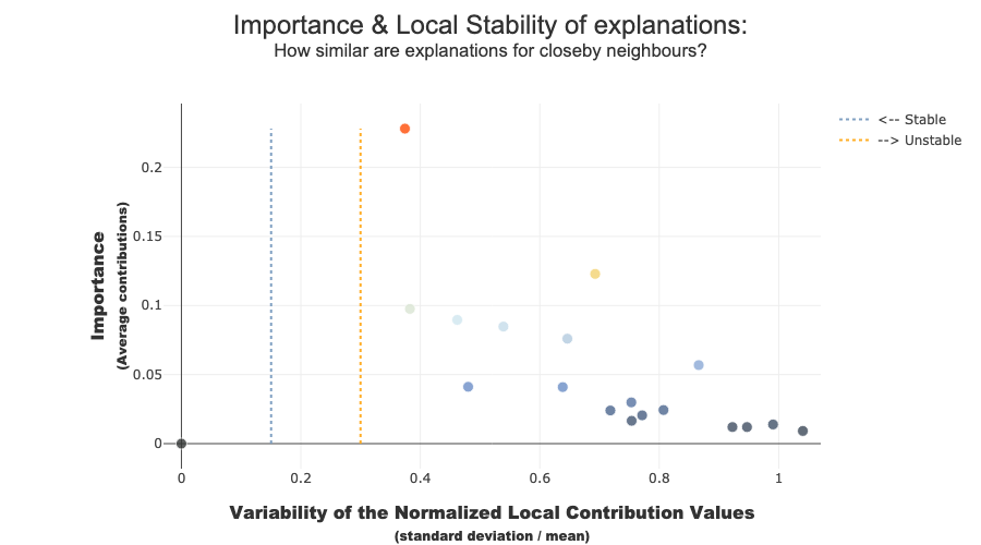
../../_images/tutorials_explainer_and_backend_tuto-expl04-Shapash-compute-Lime-faster_56_0.png

The difference in stability is small

With this use case, changing num_samples saves computation time and has little impact on explainability.

We can look impacts using distance and object Consistency(), as well as comparing stability

	n_estimators n_estimators: int, default=100 The number of trees in the forest. .. versionchanged:: 0.22 The default value of ``n_estimators`` changed from 10 to 100 in 0.22.	100
	criterion criterion: {"gini", "entropy", "log_loss"}, default="gini" The function to measure the quality of a split. Supported criteria are "gini" for the Gini impurity and "log_loss" and "entropy" both for the Shannon information gain, see :ref:`tree_mathematical_formulation`. Note: This parameter is tree-specific.	'gini'
	max_depth max_depth: int, default=None The maximum depth of the tree. If None, then nodes are expanded until all leaves are pure or until all leaves contain less than min_samples_split samples.	None
	min_samples_split min_samples_split: int or float, default=2 The minimum number of samples required to split an internal node: - If int, then consider `min_samples_split` as the minimum number. - If float, then `min_samples_split` is a fraction and `ceil(min_samples_split * n_samples)` are the minimum number of samples for each split. .. versionchanged:: 0.18 Added float values for fractions.	2
	min_samples_leaf min_samples_leaf: int or float, default=1 The minimum number of samples required to be at a leaf node. A split point at any depth will only be considered if it leaves at least ``min_samples_leaf`` training samples in each of the left and right branches. This may have the effect of smoothing the model, especially in regression. - If int, then consider `min_samples_leaf` as the minimum number. - If float, then `min_samples_leaf` is a fraction and `ceil(min_samples_leaf * n_samples)` are the minimum number of samples for each node. .. versionchanged:: 0.18 Added float values for fractions.	3
	min_weight_fraction_leaf min_weight_fraction_leaf: float, default=0.0 The minimum weighted fraction of the sum total of weights (of all the input samples) required to be at a leaf node. Samples have equal weight when sample_weight is not provided.	0.0
	max_features max_features: {"sqrt", "log2", None}, int or float, default="sqrt" The number of features to consider when looking for the best split: - If int, then consider `max_features` features at each split. - If float, then `max_features` is a fraction and `max(1, int(max_features * n_features_in_))` features are considered at each split. - If "sqrt", then `max_features=sqrt(n_features)`. - If "log2", then `max_features=log2(n_features)`. - If None, then `max_features=n_features`. .. versionchanged:: 1.1 The default of `max_features` changed from `"auto"` to `"sqrt"`. Note: the search for a split does not stop until at least one valid partition of the node samples is found, even if it requires to effectively inspect more than ``max_features`` features.	'sqrt'
	max_leaf_nodes max_leaf_nodes: int, default=None Grow trees with ``max_leaf_nodes`` in best-first fashion. Best nodes are defined as relative reduction in impurity. If None then unlimited number of leaf nodes.	None
	min_impurity_decrease min_impurity_decrease: float, default=0.0 A node will be split if this split induces a decrease of the impurity greater than or equal to this value. The weighted impurity decrease equation is the following:: N_t / N * (impurity - N_t_R / N_t * right_impurity - N_t_L / N_t * left_impurity) where ``N`` is the total number of samples, ``N_t`` is the number of samples at the current node, ``N_t_L`` is the number of samples in the left child, and ``N_t_R`` is the number of samples in the right child. ``N``, ``N_t``, ``N_t_R`` and ``N_t_L`` all refer to the weighted sum, if ``sample_weight`` is passed. .. versionadded:: 0.19	0.0
	bootstrap bootstrap: bool, default=True Whether bootstrap samples are used when building trees. If False, the whole dataset is used to build each tree.	True
	oob_score oob_score: bool or callable, default=False Whether to use out-of-bag samples to estimate the generalization score. By default, :func:`~sklearn.metrics.accuracy_score` is used. Provide a callable with signature `metric(y_true, y_pred)` to use a custom metric. Only available if `bootstrap=True`. For an illustration of out-of-bag (OOB) error estimation, see the example :ref:`sphx_glr_auto_examples_ensemble_plot_ensemble_oob.py`.	False
	n_jobs n_jobs: int, default=None The number of jobs to run in parallel. :meth:`fit`, :meth:`predict`, :meth:`decision_path` and :meth:`apply` are all parallelized over the trees. ``None`` means 1 unless in a :obj:`joblib.parallel_backend` context. ``-1`` means using all processors. See :term:`Glossary ` for more details.	None
	random_state random_state: int, RandomState instance or None, default=None Controls both the randomness of the bootstrapping of the samples used when building trees (if ``bootstrap=True``) and the sampling of the features to consider when looking for the best split at each node (if ``max_features < n_features``). See :term:`Glossary ` for details.	None
	verbose verbose: int, default=0 Controls the verbosity when fitting and predicting.	0
	warm_start warm_start: bool, default=False When set to ``True``, reuse the solution of the previous call to fit and add more estimators to the ensemble, otherwise, just fit a whole new forest. See :term:`Glossary ` and :ref:`tree_ensemble_warm_start` for details.	False
	class_weight class_weight: {"balanced", "balanced_subsample"}, dict or list of dicts, default=None Weights associated with classes in the form ``{class_label: weight}``. If not given, all classes are supposed to have weight one. For multi-output problems, a list of dicts can be provided in the same order as the columns of y. Note that for multioutput (including multilabel) weights should be defined for each class of every column in its own dict. For example, for four-class multilabel classification weights should be [{0: 1, 1: 1}, {0: 1, 1: 5}, {0: 1, 1: 1}, {0: 1, 1: 1}] instead of [{1:1}, {2:5}, {3:1}, {4:1}]. The "balanced" mode uses the values of y to automatically adjust weights inversely proportional to class frequencies in the input data as ``n_samples / (n_classes * np.bincount(y))`` The "balanced_subsample" mode is the same as "balanced" except that weights are computed based on the bootstrap sample for every tree grown. For multi-output, the weights of each column of y will be multiplied. Note that these weights will be multiplied with sample_weight (passed through the fit method) if sample_weight is specified.	None
	ccp_alpha ccp_alpha: non-negative float, default=0.0 Complexity parameter used for Minimal Cost-Complexity Pruning. The subtree with the largest cost complexity that is smaller than ``ccp_alpha`` will be chosen. By default, no pruning is performed. See :ref:`minimal_cost_complexity_pruning` for details. See :ref:`sphx_glr_auto_examples_tree_plot_cost_complexity_pruning.py` for an example of such pruning. .. versionadded:: 0.22	0.0
	max_samples max_samples: int or float, default=None If bootstrap is True, the number of samples to draw from X to train each base estimator. - If None (default), then draw `X.shape[0]` samples. - If int, then draw `max_samples` samples. - If float, then draw `max(round(n_samples * max_samples), 1)` samples. Thus, `max_samples` should be in the interval `(0.0, 1.0]`. .. versionadded:: 0.22	None
	monotonic_cst monotonic_cst: array-like of int of shape (n_features), default=None Indicates the monotonicity constraint to enforce on each feature. - 1: monotonic increase - 0: no constraint - -1: monotonic decrease If monotonic_cst is None, no constraints are applied. Monotonicity constraints are not supported for: - multiclass classifications (i.e. when `n_classes > 2`), - multioutput classifications (i.e. when `n_outputs_ > 1`), - classifications trained on data with missing values. The constraints hold over the probability of the positive class. Read more in the :ref:`User Guide `. .. versionadded:: 1.4	None