Shapash with custom colors
With this tutorial you will understand how to manipulate colors with Shapash plots
Contents: - Build a Regressor - Compile Shapash SmartExplainer - Use palette_name parameter - Use colors_dict parameter - Change the colors after comiling the explainer
Data from Kaggle House Prices
[1]:
import pandas as pd
from category_encoders import OrdinalEncoder
from lightgbm import LGBMRegressor
from sklearn.model_selection import train_test_split
Building Supervized Model
[2]:
from shapash.data.data_loader import data_loading
house_df, house_dict = data_loading('house_prices')
[3]:
y_df=house_df['SalePrice'].to_frame()
X_df=house_df[house_df.columns.difference(['SalePrice'])]
[4]:
house_df.head()
[4]:
| MSSubClass | MSZoning | LotArea | Street | LotShape | LandContour | Utilities | LotConfig | LandSlope | Neighborhood | ... | EnclosedPorch | 3SsnPorch | ScreenPorch | PoolArea | MiscVal | MoSold | YrSold | SaleType | SaleCondition | SalePrice | |
|---|---|---|---|---|---|---|---|---|---|---|---|---|---|---|---|---|---|---|---|---|---|
| Id | |||||||||||||||||||||
| 1 | 2-Story 1946 & Newer | Residential Low Density | 8450 | Paved | Regular | Near Flat/Level | All public Utilities (E,G,W,& S) | Inside lot | Gentle slope | College Creek | ... | 0 | 0 | 0 | 0 | 0 | 2 | 2008 | Warranty Deed - Conventional | Normal Sale | 208500 |
| 2 | 1-Story 1946 & Newer All Styles | Residential Low Density | 9600 | Paved | Regular | Near Flat/Level | All public Utilities (E,G,W,& S) | Frontage on 2 sides of property | Gentle slope | Veenker | ... | 0 | 0 | 0 | 0 | 0 | 5 | 2007 | Warranty Deed - Conventional | Normal Sale | 181500 |
| 3 | 2-Story 1946 & Newer | Residential Low Density | 11250 | Paved | Slightly irregular | Near Flat/Level | All public Utilities (E,G,W,& S) | Inside lot | Gentle slope | College Creek | ... | 0 | 0 | 0 | 0 | 0 | 9 | 2008 | Warranty Deed - Conventional | Normal Sale | 223500 |
| 4 | 2-Story 1945 & Older | Residential Low Density | 9550 | Paved | Slightly irregular | Near Flat/Level | All public Utilities (E,G,W,& S) | Corner lot | Gentle slope | Crawford | ... | 272 | 0 | 0 | 0 | 0 | 2 | 2006 | Warranty Deed - Conventional | Abnormal Sale | 140000 |
| 5 | 2-Story 1946 & Newer | Residential Low Density | 14260 | Paved | Slightly irregular | Near Flat/Level | All public Utilities (E,G,W,& S) | Frontage on 2 sides of property | Gentle slope | Northridge | ... | 0 | 0 | 0 | 0 | 0 | 12 | 2008 | Warranty Deed - Conventional | Normal Sale | 250000 |
5 rows × 73 columns
[5]:
from category_encoders import OrdinalEncoder

categorical_features = [col for col in X_df.columns if X_df[col].dtype == 'object']

encoder = OrdinalEncoder(
    cols=categorical_features,
    handle_unknown='ignore',
    return_df=True).fit(X_df)

X_df=encoder.transform(X_df)
[6]:
Xtrain, Xtest, ytrain, ytest = train_test_split(X_df, y_df, train_size=0.75, random_state=1)
[7]:
regressor = LGBMRegressor(n_estimators=200).fit(Xtrain,ytrain)
[LightGBM] [Info] Auto-choosing row-wise multi-threading, the overhead of testing was 0.001422 seconds.
You can set `force_row_wise=true` to remove the overhead.
And if memory is not enough, you can set `force_col_wise=true`.
[LightGBM] [Info] Total Bins 2986
[LightGBM] [Info] Number of data points in the train set: 1095, number of used features: 66
[LightGBM] [Info] Start training from score 182319.757078
[8]:
y_pred = pd.DataFrame(regressor.predict(Xtest),columns=['pred'],index=Xtest.index)
Shapash with different colors
Option 1 : use palette_name parameter
[9]:
from shapash import SmartExplainer
[10]:
xpl = SmartExplainer(
    model=regressor,
    preprocessing=encoder, # Optional: compile step can use inverse_transform method
    features_dict=house_dict,
    palette_name='blues'  # Other available name : 'default'
)
[11]:
xpl.compile(
    x=Xtest,
    y_pred=y_pred, # Optional
    y_target=ytest, # Optional: allows to display True Values vs Predicted Values
)
INFO: Shap explainer type - <shap.explainers._tree.TreeExplainer object at 0x7f1d1b7d3910>
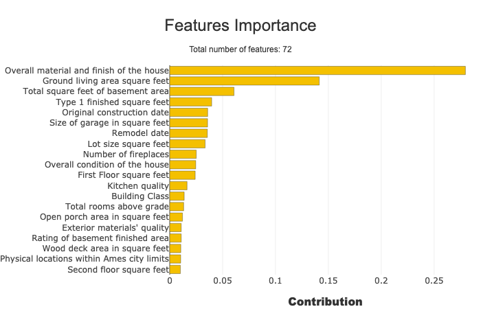
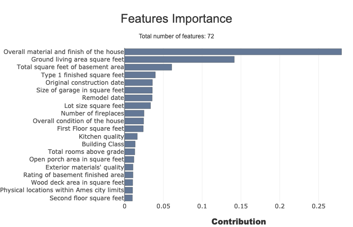
[12]:
xpl.plot.features_importance()
[12]:

Option 2 : define user-specific colors with colors_dict parameter
The colors declared will replace the one in the palette used.
In the example below, we replace the colors used in the features importance bar plot:
[13]:
# first, let's print the colors used in the previous explainer:
xpl.colors_dict['featureimp_bar']
[13]:
{'1': 'rgba(0, 154, 203, 1)', '2': 'rgba(223, 103, 0, 0.8)'}
[14]:
# Now we replace these colors using the colors_dict parameter
xpl2 = SmartExplainer(
    model=regressor,
    preprocessing=encoder,
    features_dict=house_dict,
    colors_dict=dict(
        featureimp_bar={
            '1': 'rgba(100, 120, 150, 1)',
            '2': 'rgba(120, 103, 50, 0.8)'
        },
        featureimp_line='rgba(150, 150, 54, 0.8)'
    )
)
[15]:
xpl2.compile(x=Xtest, y_pred=y_pred)
INFO: Shap explainer type - <shap.explainers._tree.TreeExplainer object at 0x7f1d1b6f0ee0>
[16]:
xpl2.plot.features_importance()
[16]:
Option 3 : redefine colors after compiling shapash
[17]:
xpl3 = SmartExplainer(
    model=regressor,
    preprocessing=encoder,
    features_dict=house_dict,
)
[18]:
xpl3.compile(x=Xtest, y_pred=y_pred)
INFO: Shap explainer type - <shap.explainers._tree.TreeExplainer object at 0x7f1d1b1fbf10>
[19]:
xpl3.plot.features_importance()
[19]:
[20]:
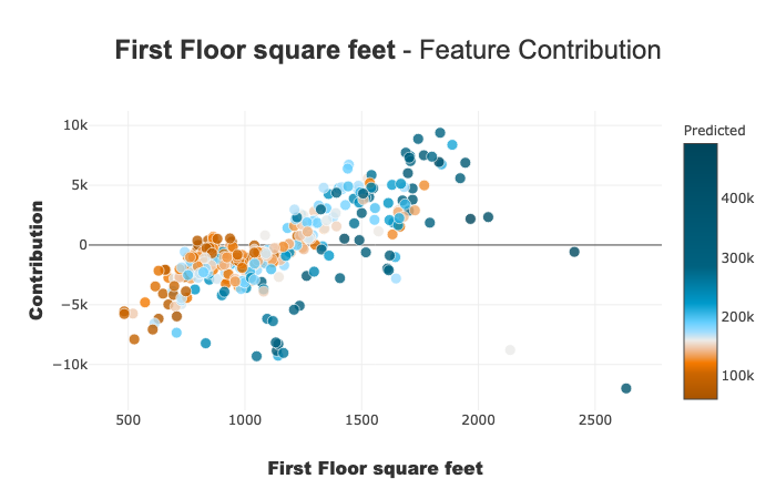
xpl3.plot.contribution_plot('1stFlrSF')
[20]:
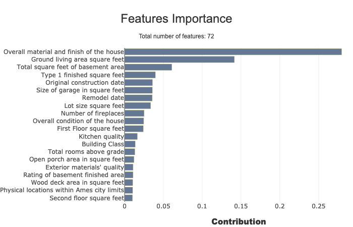
We redefine the colors with the ``blues`` palette and custom colors for the features importance plot
[21]:
xpl3.define_style(
    palette_name='blues',
    colors_dict=dict(
        featureimp_bar={
            '1': 'rgba(100, 120, 150, 1)',
            '2': 'rgba(120, 103, 50, 0.8)'
        }
))
[22]:
xpl3.plot.features_importance()
[22]:
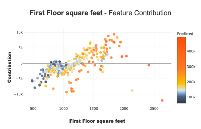
[23]:
xpl3.plot.contribution_plot('1stFlrSF')
[23]: