Shapash - Counterfactual Business Scenarios¶

This notebook shows how to compare business action scenarios for an at-risk customer and identify the best lever using local explanations.

[ ]:

import numpy as np
import pandas as pd

from category_encoders import one_hot
from sklearn.ensemble import RandomForestClassifier
from sklearn.metrics import accuracy_score, precision_score, recall_score, f1_score
from sklearn.model_selection import train_test_split

from shapash import SmartExplainer

1. Build a synthetic default target¶

We generate a synthetic consumer credit portfolio to illustrate default-risk scoring and counterfactual business scenarios. - 1: borrower likely to default - 0: borrower unlikely to default

[ ]:

rng = np.random.default_rng(42)
n_samples = 1800

df = pd.DataFrame(
    {
        "Age": rng.integers(21, 71, n_samples),
        "Income": rng.normal(55000, 18000, n_samples).clip(18000, 160000).round(0),
        "LoanAmount": rng.normal(25000, 12000, n_samples).clip(2000, 90000).round(0),
        "CreditScore": rng.normal(680, 55, n_samples).clip(480, 840).round(0),
        "EmploymentYears": rng.integers(0, 31, n_samples),
        "NumLatePayments": rng.poisson(0.9, n_samples).clip(0, 8),
        "DTI": rng.normal(0.32, 0.12, n_samples).clip(0.05, 0.8).round(3),
        "HomeOwner": rng.choice(["Yes", "No"], n_samples, p=[0.62, 0.38]),
        "MaritalStatus": rng.choice(["Single", "Married", "Divorced"], n_samples, p=[0.36, 0.52, 0.12]),
        "LoanPurpose": rng.choice(
            ["Debt consolidation", "Car purchase", "Home improvement", "Medical", "Education"],
            n_samples,
            p=[0.34, 0.19, 0.21, 0.12, 0.14],
        ),
    }
)

homeowner_flag = (df["HomeOwner"] == "Yes").astype(float)
purpose_risk = df["LoanPurpose"].map(
    {
        "Debt consolidation": 0.40,
        "Car purchase": 0.10,
        "Home improvement": 0.08,
        "Medical": 0.22,
        "Education": 0.06,
    }
)

logit = (
    -4.0
    + 3.0 * (df["LoanAmount"] / df["Income"]).astype(float)
    + 3.6 * df["DTI"].astype(float)
    + 0.018 * (700 - df["CreditScore"]).astype(float)
    + 0.65 * df["NumLatePayments"].astype(float)
    - 0.10 * df["EmploymentYears"].astype(float)
    - 0.45 * homeowner_flag
    + purpose_risk.astype(float)
    + rng.normal(0, 0.5, n_samples)
 )

default_probability = 1 / (1 + np.exp(-logit))
df["Default"] = rng.binomial(1, default_probability)

features = [
    "Age",
    "Income",
    "LoanAmount",
    "CreditScore",
    "EmploymentYears",
    "NumLatePayments",
    "DTI",
    "HomeOwner",
    "MaritalStatus",
    "LoanPurpose",
]
target_name = "Default"

X_raw = df[features]
y = df[[target_name]]

X_train_raw, X_test_raw, y_train, y_test = train_test_split(
    X_raw, y, test_size=0.25, random_state=42, stratify=y
)

encoder = one_hot.OneHotEncoder(cols=["HomeOwner", "MaritalStatus", "LoanPurpose"])
X_train = encoder.fit_transform(X_train_raw)
X_test = encoder.transform(X_test_raw)

clf = RandomForestClassifier(n_estimators=300, random_state=42, n_jobs=-1)
clf.fit(X_train, y_train.iloc[:, 0])

RandomForestClassifier(n_estimators=300, n_jobs=-1, random_state=42)

In a Jupyter environment, please rerun this cell to show the HTML representation or trust the notebook.
On GitHub, the HTML representation is unable to render, please try loading this page with nbviewer.org.

[3]:

def cls_metrics(y_true, y_pred):
    return {
        "accuracy": accuracy_score(y_true, y_pred),
        "precision": precision_score(y_true, y_pred, zero_division=0),
        "recall": recall_score(y_true, y_pred, zero_division=0),
        "f1": f1_score(y_true, y_pred, zero_division=0),
    }

pred_test = clf.predict(X_test)
metrics = pd.DataFrame([cls_metrics(y_test.iloc[:, 0], pred_test)], index=["test"])
metrics

[3]:

	accuracy	precision	recall	f1
test	0.833333	0.734375	0.447619	0.556213

2. Explain baseline model¶

[4]:

feature_dict = {
    "Age": "Age",
    "Income": "Annual income",
    "LoanAmount": "Loan amount",
    "CreditScore": "Credit score",
    "EmploymentYears": "Employment history",
    "NumLatePayments": "Late payments",
    "DTI": "Debt-to-income ratio",
    "HomeOwner": "Homeowner status",
    "MaritalStatus": "Marital status",
    "LoanPurpose": "Loan purpose",
}

xpl = SmartExplainer(
    model=clf,
    preprocessing=encoder,
    features_dict=feature_dict,
    label_dict={0: "Low default risk", 1: "High default risk"},
    title_story="Default risk scenario analysis",
)

y_pred_test_df = pd.DataFrame(clf.predict(X_test), index=X_test.index, columns=[target_name])

xpl.compile(
    x=X_test,
    y_pred=y_pred_test_df,
    y_target=y_test,
    additional_data=df.loc[X_test.index, [
        "Age",
        "Income",
        "LoanAmount",
        "CreditScore",
        "EmploymentYears",
        "NumLatePayments",
        "DTI",
        "HomeOwner",
        "MaritalStatus",
        "LoanPurpose",
    ]],
)

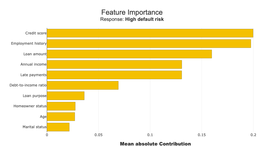
xpl.plot.features_importance()

INFO: Shap explainer type - <shap.explainers._tree.TreeExplainer object at 0x108dde000>

../../_images/tutorials_debug_and_what_if_tuto-debug03-counterfactual-business-scenarios_6_1.png

3. Pick one high-risk borrower¶

[5]:

proba_test = pd.Series(clf.predict_proba(X_test)[:, 1], index=X_test_raw.index)
customer_idx = proba_test.sort_values(ascending=False).index[0]

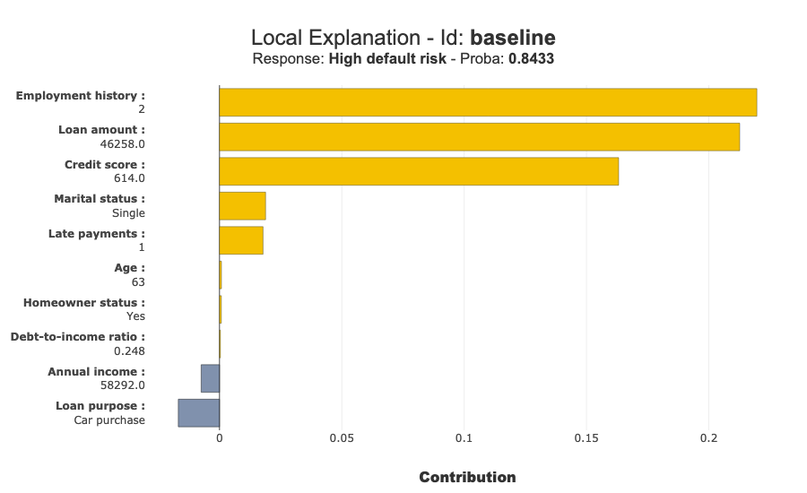
base_customer = X_test_raw.loc[[customer_idx]].copy()
base_risk = float(clf.predict_proba(encoder.transform(base_customer))[:, 1][0])

base_customer.assign(default_probability=base_risk).T

[5]:

	1705
Age	63
Income	58292.0
LoanAmount	46258.0
CreditScore	614.0
EmploymentYears	2
NumLatePayments	1
DTI	0.248
HomeOwner	Yes
MaritalStatus	Single
LoanPurpose	Car purchase
default_probability	0.843333

4. Define business scenarios (counterfactuals)¶

Simplified action rules for the demo: - loan_reduction: reduce LoanAmount by 20% - credit_repair: improve CreditScore and reduce recent late payments - income_growth: increase Income and lower DTI - full_restructure: combine all three actions

[6]:

def apply_scenario(base_row, scenario_name):
    row = base_row.copy()
    if scenario_name == "loan_reduction":
        row.loc[:, "LoanAmount"] = np.maximum(1000.0, row["LoanAmount"].fillna(25000).iloc[0] * 0.8)
        row.loc[:, "DTI"] = np.maximum(0.05, row["DTI"].fillna(0.3).iloc[0] * 0.9)
    elif scenario_name == "credit_repair":
        row.loc[:, "CreditScore"] = min(850.0, row["CreditScore"].fillna(680).iloc[0] + 40)
        row.loc[:, "NumLatePayments"] = max(0, int(row["NumLatePayments"].fillna(0).iloc[0]) - 1)
    elif scenario_name == "income_growth":
        row.loc[:, "Income"] = row["Income"].fillna(55000).iloc[0] * 1.2
        row.loc[:, "DTI"] = np.maximum(0.05, row["DTI"].fillna(0.3).iloc[0] * 0.85)
    elif scenario_name == "full_restructure":
        row.loc[:, "LoanAmount"] = np.maximum(1000.0, row["LoanAmount"].fillna(25000).iloc[0] * 0.8)
        row.loc[:, "CreditScore"] = min(850.0, row["CreditScore"].fillna(680).iloc[0] + 40)
        row.loc[:, "NumLatePayments"] = max(0, int(row["NumLatePayments"].fillna(0).iloc[0]) - 1)
        row.loc[:, "Income"] = row["Income"].fillna(55000).iloc[0] * 1.2
        row.loc[:, "DTI"] = np.maximum(0.05, row["DTI"].fillna(0.3).iloc[0] * 0.8)
    else:
        raise ValueError(f"Unknown scenario: {scenario_name}")
    return row

scenario_names = ["loan_reduction", "credit_repair", "income_growth", "full_restructure"]
scenario_rows = []

for name in scenario_names:
    row = apply_scenario(base_customer, name)
    row.index = [name]
    scenario_rows.append(row)

scenario_df = pd.concat(scenario_rows, axis=0)
scenario_proba = clf.predict_proba(encoder.transform(scenario_df))[:, 1]

result = pd.DataFrame(
    {
        "scenario": scenario_names,
        "baseline_risk": [base_risk] * len(scenario_names),
        "scenario_risk": scenario_proba,
        "risk_delta": scenario_proba - base_risk,
    }
)
result.sort_values("risk_delta")

[6]:

	scenario	baseline_risk	scenario_risk	risk_delta
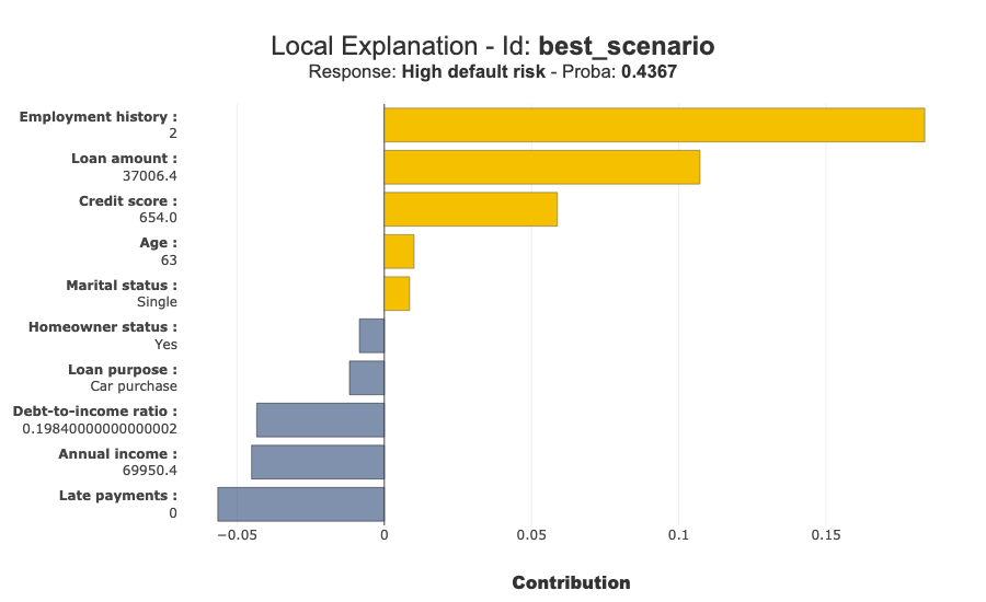
3	full_restructure	0.843333	0.436667	-0.406667
0	loan_reduction	0.843333	0.700000	-0.143333
2	income_growth	0.843333	0.713333	-0.130000
1	credit_repair	0.843333	0.740000	-0.103333

5. Explain baseline vs best scenario¶

[7]:

best_scenario_name = result.sort_values("risk_delta").iloc[0]["scenario"]
best_row = scenario_df.loc[[best_scenario_name]].copy()

compare_rows = pd.concat([base_customer, best_row], axis=0)
compare_rows.index = ["baseline", "best_scenario"]

compare_encoded = encoder.transform(compare_rows)
compare_pred_df = pd.DataFrame(
    clf.predict(compare_encoded),
    index=compare_rows.index,
    columns=[target_name],
)

xpl_compare = SmartExplainer(
    model=clf,
    preprocessing=encoder,
    features_dict=feature_dict,
    label_dict={0: "Low default risk", 1: "High default risk"},
    title_story="Counterfactual comparison",
)
xpl_compare.compile(x=compare_encoded, y_pred=compare_pred_df, additional_data=compare_rows)

xpl_compare.plot.local_plot(index="baseline")

INFO: Shap explainer type - <shap.explainers._tree.TreeExplainer object at 0x11ea85dc0>

../../_images/tutorials_debug_and_what_if_tuto-debug03-counterfactual-business-scenarios_12_1.png

[8]:

xpl_compare.plot.local_plot(index="best_scenario")

../../_images/tutorials_debug_and_what_if_tuto-debug03-counterfactual-business-scenarios_13_0.png

6. Decision checklist¶

Rank scenarios by impact and business cost.
Exclude non-actionable or sensitive variables.
Verify the plausibility of the proposed counterfactuals.
Monitor the effects actually observed after deployment.

	n_estimators n_estimators: int, default=100 The number of trees in the forest. .. versionchanged:: 0.22 The default value of ``n_estimators`` changed from 10 to 100 in 0.22.	300
	criterion criterion: {"gini", "entropy", "log_loss"}, default="gini" The function to measure the quality of a split. Supported criteria are "gini" for the Gini impurity and "log_loss" and "entropy" both for the Shannon information gain, see :ref:`tree_mathematical_formulation`. Note: This parameter is tree-specific.	'gini'
	max_depth max_depth: int, default=None The maximum depth of the tree. If None, then nodes are expanded until all leaves are pure or until all leaves contain less than min_samples_split samples.	None
	min_samples_split min_samples_split: int or float, default=2 The minimum number of samples required to split an internal node: - If int, then consider `min_samples_split` as the minimum number. - If float, then `min_samples_split` is a fraction and `ceil(min_samples_split * n_samples)` are the minimum number of samples for each split. .. versionchanged:: 0.18 Added float values for fractions.	2
	min_samples_leaf min_samples_leaf: int or float, default=1 The minimum number of samples required to be at a leaf node. A split point at any depth will only be considered if it leaves at least ``min_samples_leaf`` training samples in each of the left and right branches. This may have the effect of smoothing the model, especially in regression. - If int, then consider `min_samples_leaf` as the minimum number. - If float, then `min_samples_leaf` is a fraction and `ceil(min_samples_leaf * n_samples)` are the minimum number of samples for each node. .. versionchanged:: 0.18 Added float values for fractions.	1
	min_weight_fraction_leaf min_weight_fraction_leaf: float, default=0.0 The minimum weighted fraction of the sum total of weights (of all the input samples) required to be at a leaf node. Samples have equal weight when sample_weight is not provided.	0.0
	max_features max_features: {"sqrt", "log2", None}, int or float, default="sqrt" The number of features to consider when looking for the best split: - If int, then consider `max_features` features at each split. - If float, then `max_features` is a fraction and `max(1, int(max_features * n_features_in_))` features are considered at each split. - If "sqrt", then `max_features=sqrt(n_features)`. - If "log2", then `max_features=log2(n_features)`. - If None, then `max_features=n_features`. .. versionchanged:: 1.1 The default of `max_features` changed from `"auto"` to `"sqrt"`. Note: the search for a split does not stop until at least one valid partition of the node samples is found, even if it requires to effectively inspect more than ``max_features`` features.	'sqrt'
	max_leaf_nodes max_leaf_nodes: int, default=None Grow trees with ``max_leaf_nodes`` in best-first fashion. Best nodes are defined as relative reduction in impurity. If None then unlimited number of leaf nodes.	None
	min_impurity_decrease min_impurity_decrease: float, default=0.0 A node will be split if this split induces a decrease of the impurity greater than or equal to this value. The weighted impurity decrease equation is the following:: N_t / N * (impurity - N_t_R / N_t * right_impurity - N_t_L / N_t * left_impurity) where ``N`` is the total number of samples, ``N_t`` is the number of samples at the current node, ``N_t_L`` is the number of samples in the left child, and ``N_t_R`` is the number of samples in the right child. ``N``, ``N_t``, ``N_t_R`` and ``N_t_L`` all refer to the weighted sum, if ``sample_weight`` is passed. .. versionadded:: 0.19	0.0
	bootstrap bootstrap: bool, default=True Whether bootstrap samples are used when building trees. If False, the whole dataset is used to build each tree.	True
	oob_score oob_score: bool or callable, default=False Whether to use out-of-bag samples to estimate the generalization score. By default, :func:`~sklearn.metrics.accuracy_score` is used. Provide a callable with signature `metric(y_true, y_pred)` to use a custom metric. Only available if `bootstrap=True`. For an illustration of out-of-bag (OOB) error estimation, see the example :ref:`sphx_glr_auto_examples_ensemble_plot_ensemble_oob.py`.	False
	n_jobs n_jobs: int, default=None The number of jobs to run in parallel. :meth:`fit`, :meth:`predict`, :meth:`decision_path` and :meth:`apply` are all parallelized over the trees. ``None`` means 1 unless in a :obj:`joblib.parallel_backend` context. ``-1`` means using all processors. See :term:`Glossary ` for more details.	-1
	random_state random_state: int, RandomState instance or None, default=None Controls both the randomness of the bootstrapping of the samples used when building trees (if ``bootstrap=True``) and the sampling of the features to consider when looking for the best split at each node (if ``max_features < n_features``). See :term:`Glossary ` for details.	42
	verbose verbose: int, default=0 Controls the verbosity when fitting and predicting.	0
	warm_start warm_start: bool, default=False When set to ``True``, reuse the solution of the previous call to fit and add more estimators to the ensemble, otherwise, just fit a whole new forest. See :term:`Glossary ` and :ref:`tree_ensemble_warm_start` for details.	False
	class_weight class_weight: {"balanced", "balanced_subsample"}, dict or list of dicts, default=None Weights associated with classes in the form ``{class_label: weight}``. If not given, all classes are supposed to have weight one. For multi-output problems, a list of dicts can be provided in the same order as the columns of y. Note that for multioutput (including multilabel) weights should be defined for each class of every column in its own dict. For example, for four-class multilabel classification weights should be [{0: 1, 1: 1}, {0: 1, 1: 5}, {0: 1, 1: 1}, {0: 1, 1: 1}] instead of [{1:1}, {2:5}, {3:1}, {4:1}]. The "balanced" mode uses the values of y to automatically adjust weights inversely proportional to class frequencies in the input data as ``n_samples / (n_classes * np.bincount(y))`` The "balanced_subsample" mode is the same as "balanced" except that weights are computed based on the bootstrap sample for every tree grown. For multi-output, the weights of each column of y will be multiplied. Note that these weights will be multiplied with sample_weight (passed through the fit method) if sample_weight is specified.	None
	ccp_alpha ccp_alpha: non-negative float, default=0.0 Complexity parameter used for Minimal Cost-Complexity Pruning. The subtree with the largest cost complexity that is smaller than ``ccp_alpha`` will be chosen. By default, no pruning is performed. See :ref:`minimal_cost_complexity_pruning` for details. See :ref:`sphx_glr_auto_examples_tree_plot_cost_complexity_pruning.py` for an example of such pruning. .. versionadded:: 0.22	0.0
	max_samples max_samples: int or float, default=None If bootstrap is True, the number of samples to draw from X to train each base estimator. - If None (default), then draw `X.shape[0]` samples. - If int, then draw `max_samples` samples. - If float, then draw `max(round(n_samples * max_samples), 1)` samples. Thus, `max_samples` should be in the interval `(0.0, 1.0]`. .. versionadded:: 0.22	None
	monotonic_cst monotonic_cst: array-like of int of shape (n_features), default=None Indicates the monotonicity constraint to enforce on each feature. - 1: monotonic increase - 0: no constraint - -1: monotonic decrease If monotonic_cst is None, no constraints are applied. Monotonicity constraints are not supported for: - multiclass classifications (i.e. when `n_classes > 2`), - multioutput classifications (i.e. when `n_outputs_ > 1`), - classifications trained on data with missing values. The constraints hold over the probability of the positive class. Read more in the :ref:`User Guide `. .. versionadded:: 1.4	None