How to use filter and local_plot methods

This tutorial presents the different parameters you can use to summarize and display local explanations. It also shows how to export this summary into pandas DataFrame

Contents: - Work with filter and local_plot method to tune output - display Positive or Negative contributions - mask hidden contrib or prediction - hide some specific features - Use query parameter to select without index or row number - Classification: How can you select the label value to display? - print the summary params - export local explanation with to_pandas

Data from Kaggle House Prices

import pandas as pd
from category_encoders import OrdinalEncoder
from catboost import CatBoostRegressor, CatBoostClassifier
from sklearn.model_selection import train_test_split

Building Supervized Model

from shapash.data.data_loader import data_loading
house_df, house_dict = data_loading('house_prices')
y_df=house_df['SalePrice'].to_frame()
X_df=house_df[house_df.columns.difference(['SalePrice'])]

from category_encoders import OrdinalEncoder

categorical_features = [col for col in X_df.columns if X_df[col].dtype == 'object']

encoder = OrdinalEncoder(
    cols=categorical_features,
    handle_unknown='ignore',
    return_df=True).fit(X_df)

X_df=encoder.transform(X_df)

Xtrain, Xtest, ytrain, ytest = train_test_split(X_df, y_df, train_size=0.75, random_state=1)

regressor = CatBoostRegressor(n_estimators=50).fit(Xtrain,ytrain,verbose=False)

y_pred = pd.DataFrame(regressor.predict(Xtest),columns=['pred'],index=Xtest.index)

Work With filter and local_plot methods

First step: You need to Declare and Compile SmartExplainer

from shapash import SmartExplainer

xpl = SmartExplainer(
    model=regressor,
    preprocessing=encoder, # Optional: compile step can use inverse_transform method
    features_dict=house_dict, # Optional parameter, dict specifies label for features name
)

xpl.compile(
    x=Xtest,
    y_pred=y_pred # Optional
)

Backend: Shap TreeExplainer

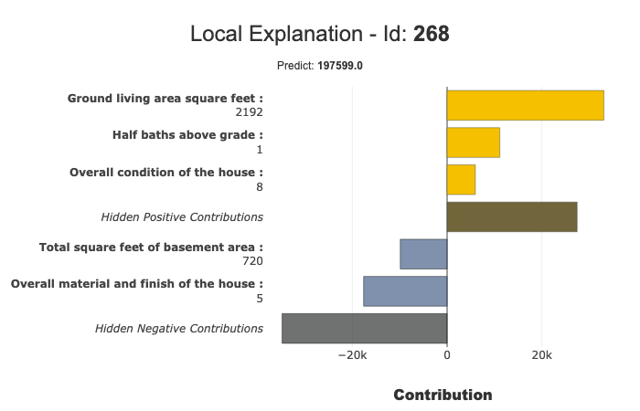
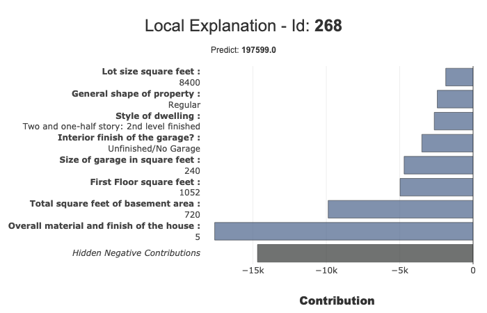
Filter method

Use the filter method to specify how to summarize local explainability you have 4 parameters to customize your summary: - max_contrib : maximum number of criteria to display - threshold : minimum value of the contribution (in absolute value) necessary to display a criterion - positive : display only positive contribution? Negative?(default None) - features_to_hide : list of features you don’t want to display

xpl.filter(max_contrib=5)

Local_plot

xpl.plot.local_plot(index=268)

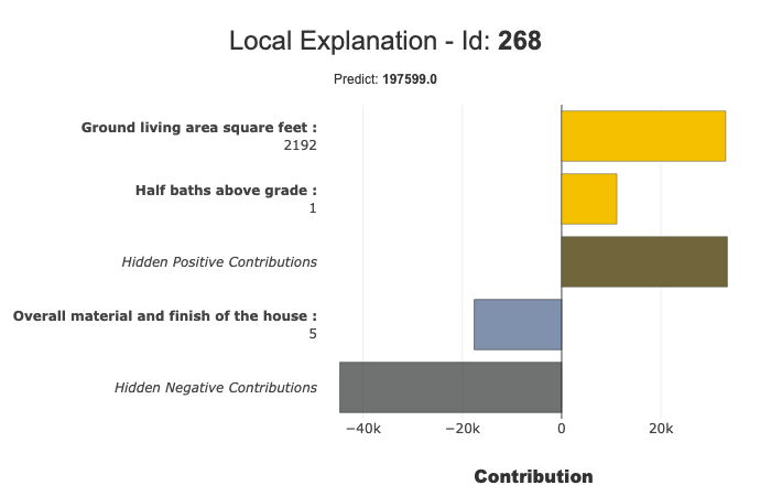
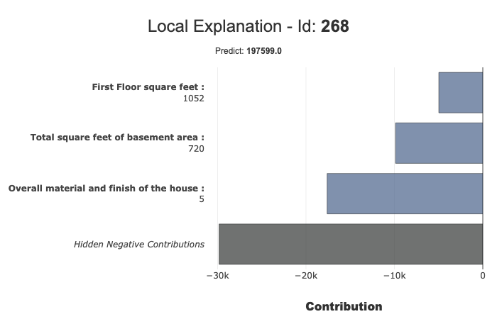
Threshold parameter to focus on significant contributions

xpl.filter(max_contrib=5,threshold=10000)
xpl.plot.local_plot(index=268)

Don’t display hidden contributions

xpl.plot.local_plot(index=268,show_masked=False)

You can also hide the predict value with parameter show_predict=False

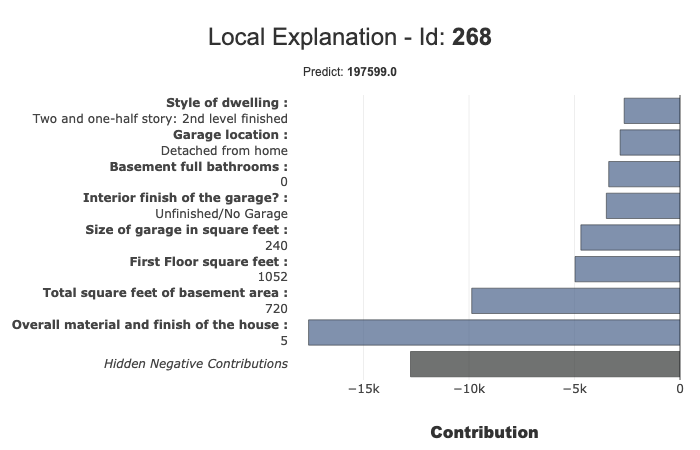
Focus on Negative contribution

xpl.filter(max_contrib=8,positive=False)
xpl.plot.local_plot(index=268)

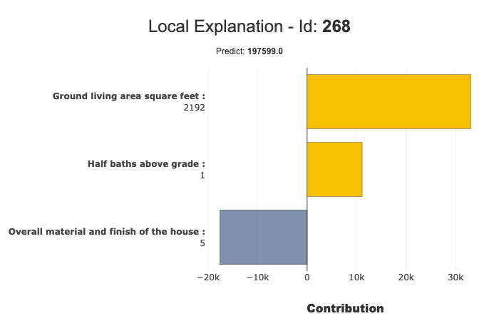
You can also focus positive contribution using positive=True

Hide specific features:

Because: - some features can be too complex - end user don’t want know unnecessary information

You can use features_to_hide parameter in filter method

xpl.filter(max_contrib=8,positive=False,features_to_hide=['BsmtFullBath','GarageType'])
xpl.plot.local_plot(index=268)

Select a row with a query

You can selct with an index or a row number. You can also use a query:

xpl.filter(max_contrib=3,positive=False)
xpl.plot.local_plot(query="LotArea == 8400 and LotShape == 'Regular' and TotalBsmtSF == 720")

Classification Case

transform our use case into classification:

ytrain['PriceClass'] = ytrain['SalePrice'].apply(lambda x: 1 if x < 150000 else (3 if x > 300000 else 2))
label_dict = { 1 : 'Cheap', 2 : 'Moderately Expensive', 3 : 'Expensive' }

clf = CatBoostClassifier(n_estimators=50).fit(Xtrain,ytrain['PriceClass'],verbose=False)
y_pred_clf = pd.DataFrame(clf.predict(Xtest),columns=['pred'],index=Xtest.index)

Declare new SmartExplainer dedicated to classification problem

xplclf = SmartExplainer(
    model=clf,
    preprocessing=encoder,
    features_dict=house_dict,
    label_dict=label_dict # Optional parameters: display explicit output
)

xplclf.compile(
    x=Xtest,
    y_pred=y_pred_clf
)

Backend: Shap TreeExplainer

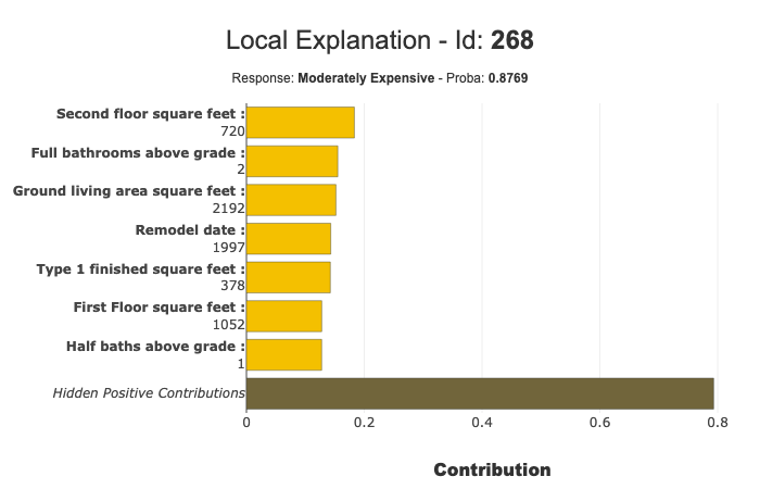
Use label parameter of local_plot parameter to select the explanation you want

with label parameter, you can specify explicit label or label number

xplclf.filter(max_contrib=7,positive=True)
xplclf.plot.local_plot(index=268,label='Moderately Expensive')

See the summary parameters

xplclf.mask_params

{'features_to_hide': None,
 'threshold': None,
 'positive': True,
 'max_contrib': 7}

Export explanations

Export your local explanation in pd.DataFrame with to_pandas method :

• The to_pandas method has the same parameters as the filter method

• if you don’t specify any parameter, to_pandas use the same params you specified when you call filter method

• When you work on classification problem, parameter proba=True output predict probability

summary_df= xplclf.to_pandas(proba=True)

to_pandas params: {'features_to_hide': None, 'threshold': None, 'positive': True, 'max_contrib': 7}

summary_df.head()

	pred	proba	feature_1	value_1	contribution_1	feature_2	value_2	contribution_2	feature_3	value_3	...	contribution_4	feature_5	value_5	contribution_5	feature_6	value_6	contribution_6	feature_7	value_7	contribution_7
259	Moderately Expensive	0.994917	Ground living area square feet	1792	0.309308	Interior finish of the garage?	Rough Finished	0.275467	Size of garage in square feet	564	...	0.182722	Physical locations within Ames city limits	College Creek	0.170888	Overall material and finish of the house	7	0.164045	Height of the basement	Good (90-99 inches)	0.139618
268	Moderately Expensive	0.876916	Second floor square feet	720	0.183251	Full bathrooms above grade	2	0.155086	Ground living area square feet	2192	...	0.143119	Type 1 finished square feet	378	0.142439	First Floor square feet	1052	0.127817	Half baths above grade	1	0.127717
289	Cheap	0.997304	Ground living area square feet	900	0.818922	Size of garage in square feet	280	0.561631	Total square feet of basement area	882	...	0.349033	Full bathrooms above grade	1	0.324806	Overall material and finish of the house	5	0.318031	First Floor square feet	900	0.247826
650	Cheap	0.998653	Ground living area square feet	630	0.816398	Size of garage in square feet	0	0.587745	Total square feet of basement area	630	...	0.355685	Overall material and finish of the house	4	0.317549	Full bathrooms above grade	1	0.31303	General zoning classification	Residential Medium Density	0.178395
1234	Cheap	0.852389	Ground living area square feet	1188	0.942118	Remodel date	1959	0.423368	Overall material and finish of the house	5	...	0.373812	Number of fireplaces	0	0.168725	Rating of basement finished area	Average Rec Room	0.130175	Wood deck area in square feet	0	0.12249

5 rows × 23 columns

It is also possible to calculate the probability relating to one of the target modality for all the dataset, and to display the elements of explainability associated with this target modality

#Create One column pd.DataFrame with constant value
constantpred=pd.DataFrame([3 for x in range(Xtest.shape[0])],columns=['pred'],index=Xtest.index)
xplclf.add(y_pred=constantpred)
summary_df = xplclf.to_pandas(proba=True,max_contrib=3,threshold=0.1,positive=True)

summary_df.head()

	pred	proba	feature_1	value_1	contribution_1	feature_2	value_2	contribution_2	feature_3	value_3	contribution_3
259	Expensive	0.003081	Ground living area square feet	1792	0.327986	Overall material and finish of the house	7	0.197494	Rating of basement finished area	Good Living Quarters	0.181953
268	Expensive	0.007627	Ground living area square feet	2192	0.825571	Wood deck area in square feet	262	0.251474	Remodel date	1997	0.157067
289	Expensive	0.000024	NaN	NaN	NaN	NaN	NaN	NaN	NaN	NaN	NaN
650	Expensive	0.000056	NaN	NaN	NaN	NaN	NaN	NaN	NaN	NaN	NaN
1234	Expensive	0.000623	Type of sale	Court Officer Deed/Estate	0.114506	NaN	NaN	NaN	NaN	NaN	NaN

NB: The to_pandas method returns Nan for lines that do not meet your conditions