Shapash + Keras in Jupyter: Titanic Survival Classification

This tutorial shows how to: - train a tabular deep learning model (Keras) - predict Titanic passenger survival - explain predictions in a notebook with Shapash

1. Imports

import numpy as np
import pandas as pd
import matplotlib.pyplot as plt

from IPython.display import clear_output, display

from category_encoders import one_hot
from sklearn.metrics import accuracy_score, classification_report
from sklearn.model_selection import train_test_split

import keras
from keras import layers

from shapash import SmartExplainer
from shapash.data.data_loader import data_loading

2. Loading the Titanic data

titanic_df, titanic_dict = data_loading('titanic')
titanic_df.head()

	Survived	Pclass	Name	Sex	Age	SibSp	Parch	Fare	Embarked	Title
PassengerId
1	0	Third class	Braund Owen Harris	male	22.0	1	0	7.25	Southampton	Mr
2	1	First class	Cumings John Bradley (Florence Briggs Thayer)	female	38.0	1	0	71.28	Cherbourg	Mrs
3	1	Third class	Heikkinen Laina	female	26.0	0	0	7.92	Southampton	Miss
4	1	First class	Futrelle Jacques Heath (Lily May Peel)	female	35.0	1	0	53.10	Southampton	Mrs
5	0	Third class	Allen William Henry	male	35.0	0	0	8.05	Southampton	Mr

features = ['Pclass', 'Age', 'Sex', 'SibSp', 'Parch', 'Fare', 'Embarked']
target = 'Survived'

df = titanic_df[features + [target]].copy()

# Convert Pclass labels to ordinal values
pclass_map = {
    'First class': 1,
    'Second class': 2,
    'Third class': 3,
}
df['Pclass'] = df['Pclass'].map(pclass_map).fillna(df['Pclass'])
df['Pclass'] = pd.to_numeric(df['Pclass'], errors='coerce')

# Clean minimal values for a tabular neural network
df['Age'] = df['Age'].fillna(df['Age'].median())
df['Fare'] = df['Fare'].fillna(df['Fare'].median())
df['Embarked'] = df['Embarked'].fillna(df['Embarked'].mode()[0])
df['Pclass'] = df['Pclass'].fillna(df['Pclass'].median())

X = df[features]
y = df[target].astype(int).to_frame()

X.shape, y.shape

((891, 7), (891, 1))

3. Encoding categorical variables

encoder = one_hot.OneHotEncoder(cols=['Sex', 'Embarked'], use_cat_names=True)
X_enc = encoder.fit_transform(X)

X_train, X_test, y_train, y_test = train_test_split(
    X_enc, y,
    test_size=0.25,
    random_state=42,
    stratify=y
)

X_train.shape, X_test.shape

((668, 10), (223, 10))

4. Deep learning model with Keras

keras.utils.set_random_seed(42)

model = keras.Sequential([
    layers.Input(shape=(X_train.shape[1],)),
    layers.Dense(64, activation='relu'),
    layers.Dropout(0.2),
    layers.Dense(32, activation='relu'),
    layers.Dense(1, activation='sigmoid')
])

model.compile(
    optimizer=keras.optimizers.Adam(learning_rate=1e-3),
    loss='binary_crossentropy',
    metrics=['accuracy'],
)

early_stopping = keras.callbacks.EarlyStopping(
    monitor='val_loss',
    patience=15,
    restore_best_weights=True
)

SHAPASH_YELLOW = '#f4c000'
SHAPASH_GREY = '#343736'

class LiveLossPlot(keras.callbacks.Callback):
    def on_train_begin(self, logs=None):
        self.train_losses = []
        self.val_losses = []

    def on_epoch_end(self, epoch, logs=None):
        logs = logs or {}
        self.train_losses.append(logs.get('loss'))
        self.val_losses.append(logs.get('val_loss'))

        fig, ax = plt.subplots(figsize=(8, 4))
        ax.plot(self.train_losses, label='Train loss', color=SHAPASH_YELLOW, linewidth=2.5)
        ax.plot(self.val_losses, label='Validation loss', color=SHAPASH_GREY, linewidth=2.5)
        ax.set_title(f'Learning curve (epoch {epoch + 1})')
        ax.set_xlabel('Epoch')
        ax.set_ylabel('Binary crossentropy loss')
        ax.grid(alpha=0.25)
        ax.legend()
        fig.tight_layout()

        clear_output(wait=True)
        display(fig)
        plt.close(fig)

live_plot = LiveLossPlot()

history = model.fit(
    X_train.values,
    y_train.values,
    validation_data=(X_test.values, y_test.values),
    epochs=200,
    batch_size=32,
    callbacks=[early_stopping, live_plot],
    # verbose=0
)
# load the best model weights from early stopping
print(f"Best val_accuracy: {max(history.history['val_accuracy']):.4f}")

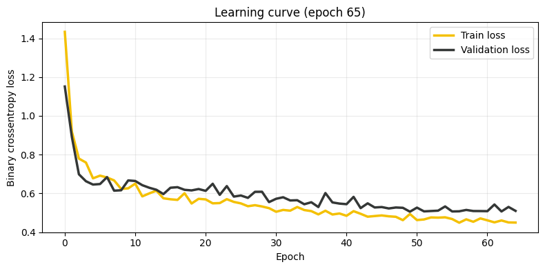
21/21 ━━━━━━━━━━━━━━━━━━━━ 0s 3ms/step - accuracy: 0.7979 - loss: 0.4499 - val_accuracy: 0.7803 - val_loss: 0.5101
Best val_accuracy: 0.7937

proba_test = model.predict(X_test.values, verbose=0).reshape(-1)
pred_test = (proba_test >= 0.5).astype(int)

print(f"Test accuracy: {accuracy_score(y_test.values.reshape(-1), pred_test):.4f}")
print(classification_report(y_test.values.reshape(-1), pred_test, digits=4))

Test accuracy: 0.7892
              precision    recall  f1-score   support

           0     0.8082    0.8613    0.8339       137
           1     0.7532    0.6744    0.7117        86

    accuracy                         0.7892       223
   macro avg     0.7807    0.7679    0.7728       223
weighted avg     0.7870    0.7892    0.7868       223

5. Sklearn-like wrapper for Shapash

Shapash detects classification with the classes_ and predict_proba attributes. We add a lightweight wrapper around the Keras model.

class KerasBinaryClassifierWrapper:
    def __init__(self, keras_model, threshold=0.5):
        self.keras_model = keras_model
        self.threshold = threshold
        self.classes_ = np.array([0, 1])
        self._classes = [0, 1]

    def predict_proba(self, X):
        p1 = self.keras_model.predict(np.asarray(X), verbose=0).reshape(-1)
        p0 = 1.0 - p1
        return np.column_stack([p0, p1])

    def predict(self, X):
        p1 = self.predict_proba(X)[:, 1]
        return (p1 >= self.threshold).astype(int)

wrapped_model = KerasBinaryClassifierWrapper(keras_model=model, threshold=0.5)

6. Compiling SmartExplainer

We use the shap backend here to keep computation time reasonable for a tabular deep learning model.

# Keep explanation runtime low for a notebook demo
n_explain = min(200, len(X_test))
X_explain = X_test.sample(n=n_explain, random_state=42)
y_target_explain = y_test.loc[X_explain.index]

y_pred = pd.DataFrame(
    wrapped_model.predict(X_explain),
    index=X_explain.index,
    columns=['Survived']
)

response_dict = {0: 'Deceased', 1: 'Survived'}

xpl = SmartExplainer(
    model=wrapped_model,
    preprocessing=encoder,
    features_dict=titanic_dict,
    label_dict=response_dict,
    backend='shap',
    title_story='Titanic survival with a Keras'
)

xpl.compile(
    x=X_explain,
    y_pred=y_pred,
    y_target=y_target_explain
)

INFO: Shap explainer type - <shap.explainers._exact.ExactExplainer object at 0x12e970440>

ExactExplainer explainer: 201it [00:55,  3.10it/s]

7. Shapash plots in the notebook

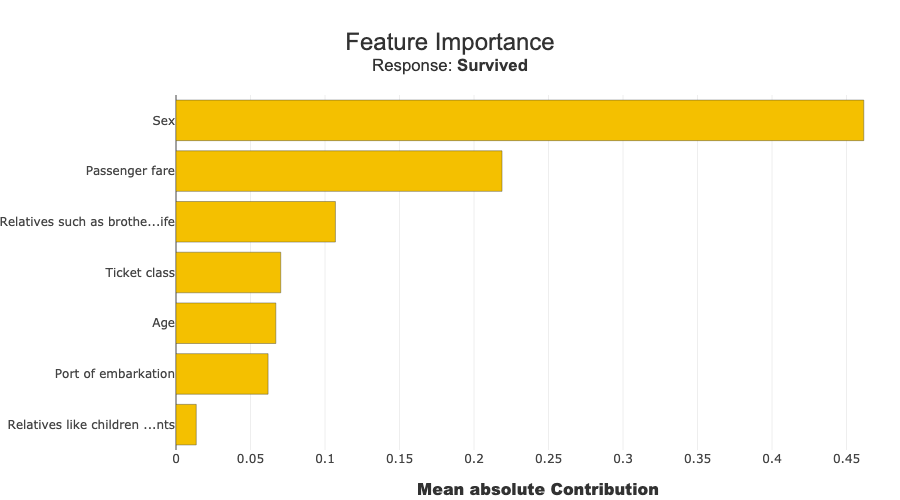
xpl.plot.features_importance()

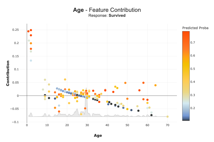
xpl.plot.contribution_plot('Age')

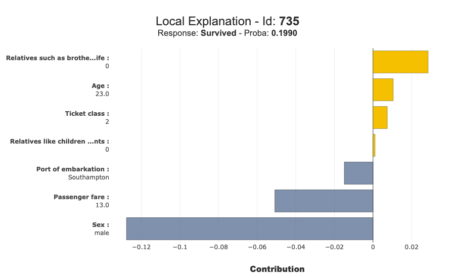
row_id = X_explain.index[0]
xpl.plot.local_plot(index=row_id)

xpl.to_pandas(max_contrib=8).head(10)

	Survived	feature_1	value_1	contribution_1	feature_2	value_2	contribution_2	feature_3	value_3	contribution_3	...	contribution_4	feature_5	value_5	contribution_5	feature_6	value_6	contribution_6	feature_7	value_7	contribution_7
735	Deceased	Sex	male	0.127684	Passenger fare	13.0	0.050851	Relatives such as brother or wife	0	-0.028539	...	0.014882	Age	23.0	-0.010472	Ticket class	2	-0.007397	Relatives like children or parents	0	-0.001051
625	Deceased	Sex	male	0.116236	Relatives such as brother or wife	0	-0.028845	Ticket class	3	0.025976	...	0.021563	Age	21.0	-0.017173	Port of embarkation	Southampton	0.014301	Relatives like children or parents	0	-0.000764
104	Deceased	Sex	male	0.125619	Passenger fare	8.65	0.088861	Relatives such as brother or wife	0	-0.025193	...	0.020886	Port of embarkation	Southampton	0.013359	Age	33.0	0.012455	Relatives like children or parents	0	-0.000961
388	Survived	Sex	female	0.286759	Relatives such as brother or wife	0	0.032435	Passenger fare	13.0	-0.023769	...	-0.014274	Ticket class	2	0.011565	Relatives like children or parents	0	0.006016	Age	36.0	0.002935
342	Survived	Sex	female	0.206648	Relatives such as brother or wife	3	-0.121622	Passenger fare	263.0	0.106484	...	0.015445	Port of embarkation	Southampton	-0.010942	Age	24.0	-0.008412	Relatives like children or parents	2	0.005304
352	Deceased	Sex	male	0.115636	Passenger fare	35.0	-0.064915	Ticket class	1	-0.048789	...	-0.031078	Port of embarkation	Southampton	0.011676	Relatives like children or parents	0	-0.004565	Age	29.5	0.002919
367	Survived	Sex	female	0.244876	Passenger fare	75.25	0.170982	Ticket class	1	0.05393	...	0.038142	Age	60.0	-0.01554	Relatives such as brother or wife	1	-0.008888	Relatives like children or parents	0	0.004335
296	Deceased	Sex	male	0.10905	Ticket class	1	-0.045848	Passenger fare	27.72	-0.035266	...	-0.030661	Port of embarkation	Cherbourg	-0.030228	Relatives like children or parents	0	-0.004339	Age	29.5	0.004128
428	Survived	Sex	female	0.242509	Relatives such as brother or wife	0	0.040903	Passenger fare	26.0	0.026343	...	0.023752	Port of embarkation	Southampton	-0.011517	Ticket class	2	0.011443	Relatives like children or parents	0	0.004754
824	Survived	Sex	female	0.266229	Relatives such as brother or wife	0	0.03253	Passenger fare	12.48	-0.031449	...	-0.025467	Port of embarkation	Southampton	-0.013692	Relatives like children or parents	1	-0.008707	Age	27.0	0.005659

10 rows × 22 columns

8. (Optional) Launch the Shapash WebApp

As in shapash/webapp/webapp_launch.py, you can also launch the interactive application:

xpl.init_app()
app = xpl.smartapp.app
app.run_server(host='localhost', port=8050)