
Shapash - Time Series Tabular Forecasting
This notebook illustrates tabular forecasting: lag creation, calendar features, then local and global interpretation with Shapash.
[ ]:
import numpy as np
import pandas as pd

from sklearn.ensemble import RandomForestRegressor
from sklearn.metrics import mean_absolute_error, r2_score

from shapash import SmartExplainer
1. Build a synthetic daily demand signal
[2]:
rng = np.random.default_rng(42)
date_index = pd.date_range(start="2021-01-01", periods=900, freq="D")

trend = np.linspace(0, 25, len(date_index))
weekly = 10 * np.sin(2 * np.pi * np.arange(len(date_index)) / 7)
yearly = 20 * np.sin(2 * np.pi * np.arange(len(date_index)) / 365)
noise = rng.normal(0, 4, len(date_index))

target = 120 + trend + weekly + yearly + noise
ts_df = pd.DataFrame({"date": date_index, "target": target})
ts_df.head()
[2]:
| date | target | |
|---|---|---|
| 0 | 2021-01-01 | 121.218868 |
| 1 | 2021-01-02 | 124.030454 |
| 2 | 2021-01-03 | 133.495133 |
| 3 | 2021-01-04 | 129.216916 |
| 4 | 2021-01-05 | 109.344305 |
2. Engineer tabular features (lags + calendar)
[3]:
df = ts_df.copy()
df["lag_1"] = df["target"].shift(1)
df["lag_7"] = df["target"].shift(7)
df["rolling_mean_7"] = df["target"].shift(1).rolling(7).mean()
df["rolling_std_7"] = df["target"].shift(1).rolling(7).std()
df["day_of_week"] = df["date"].dt.dayofweek
df["month"] = df["date"].dt.month
df["is_weekend"] = (df["day_of_week"] >= 5).astype(int)

model_df = df.dropna().reset_index(drop=True)
feature_cols = [
    "lag_1",
    "lag_7",
    "rolling_mean_7",
    "rolling_std_7",
    "day_of_week",
    "month",
    "is_weekend",
]

X = model_df[feature_cols]
y = model_df[["target"]]

split_idx = int(len(model_df) * 0.8)
X_train, X_test = X.iloc[:split_idx], X.iloc[split_idx:]
y_train, y_test = y.iloc[:split_idx], y.iloc[split_idx:]
date_train = model_df["date"].iloc[:split_idx]
date_test = model_df["date"].iloc[split_idx:]

X_train.head()
[3]:
| lag_1 | lag_7 | rolling_mean_7 | rolling_std_7 | day_of_week | month | is_weekend | |
|---|---|---|---|---|---|---|---|
| 0 | 114.921933 | 121.218868 | 119.875422 | 9.963461 | 4 | 1 | 0 |
| 1 | 121.333851 | 124.030454 | 119.891848 | 9.966140 | 5 | 1 | 1 |
| 2 | 130.719155 | 133.495133 | 120.847377 | 10.721123 | 6 | 1 | 1 |
| 3 | 129.673558 | 129.216916 | 120.301437 | 10.045764 | 0 | 1 | 0 |
| 4 | 131.560379 | 109.344305 | 120.636218 | 10.424313 | 1 | 1 | 0 |
3. Train and evaluate
[4]:
model = RandomForestRegressor(n_estimators=400, random_state=42, n_jobs=-1)
model.fit(X_train, y_train.iloc[:, 0])

pred_train = model.predict(X_train)
pred_test = model.predict(X_test)

metrics = pd.DataFrame(
    {
        "MAE": [
            mean_absolute_error(y_train.iloc[:, 0], pred_train),
            mean_absolute_error(y_test.iloc[:, 0], pred_test),
        ],
        "R2": [
            r2_score(y_train.iloc[:, 0], pred_train),
            r2_score(y_test.iloc[:, 0], pred_test),
        ],
    },
    index=["train", "test"],
)
metrics
[4]:
| MAE | R2 | |
|---|---|---|
| train | 1.511569 | 0.985118 |
| test | 5.771074 | 0.535060 |
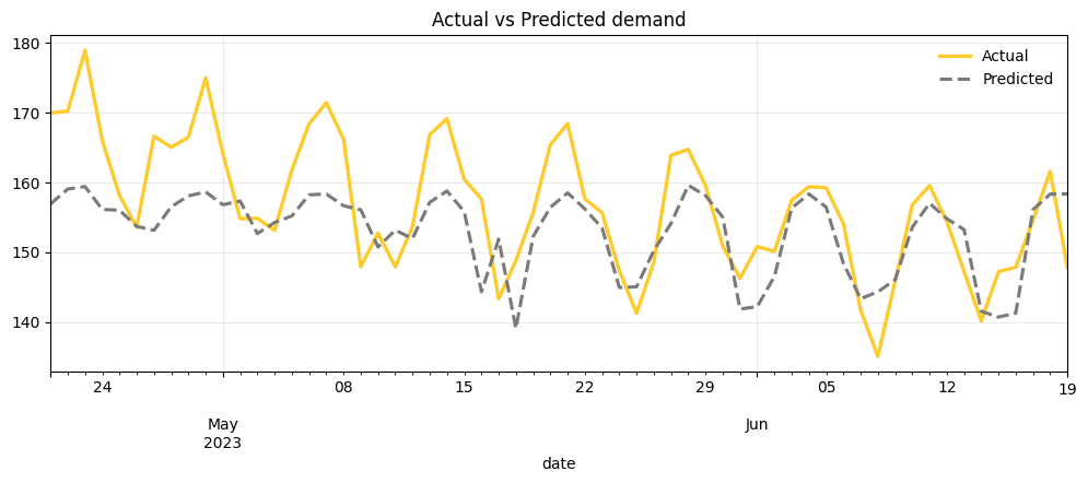
[5]:
compare_df = pd.DataFrame(
    {
        "date": date_test.values,
        "actual": y_test.iloc[:, 0].values,
        "predicted": pred_test,
    }
)

plot_df = compare_df.set_index("date").tail(60)

ax = plot_df["actual"].plot(
    figsize=(12, 4),
    color="#FECB2F",   # jaune style Shapash
    linewidth=2.4,
    label="Actual",
)
plot_df["predicted"].plot(
    ax=ax,
    color="#7A7A7A",   # gris
    linewidth=2.2,
    linestyle="--",
    label="Predicted",
)

ax.set_title("Actual vs Predicted demand")
ax.grid(alpha=0.25)
ax.legend(frameon=False)
[5]:
<matplotlib.legend.Legend at 0x1218a0110>
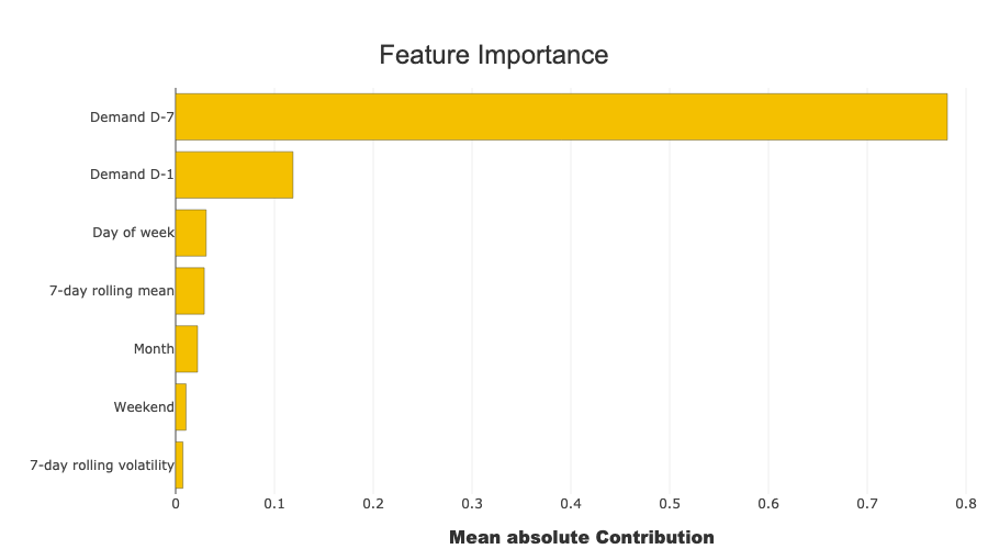
4. Explain forecasting drivers with Shapash
[6]:
feature_dict = {
    "lag_1": "Demand D-1",
    "lag_7": "Demand D-7",
    "rolling_mean_7": "7-day rolling mean",
    "rolling_std_7": "7-day rolling volatility",
    "day_of_week": "Day of week",
    "month": "Month",
    "is_weekend": "Weekend",
}

xpl = SmartExplainer(
    model=model,
    features_dict=feature_dict,
    title_story="Demand forecasting with tabular features",
)

y_pred_test_df = pd.DataFrame(pred_test, columns=["target"], index=X_test.index)

xpl.compile(
    x=X_test,
    y_pred=y_pred_test_df,
    y_target=y_test,
    additional_data=model_df.loc[X_test.index, ["date"]],
)

xpl.plot.features_importance()
INFO: Shap explainer type - <shap.explainers._tree.TreeExplainer object at 0x121857410>
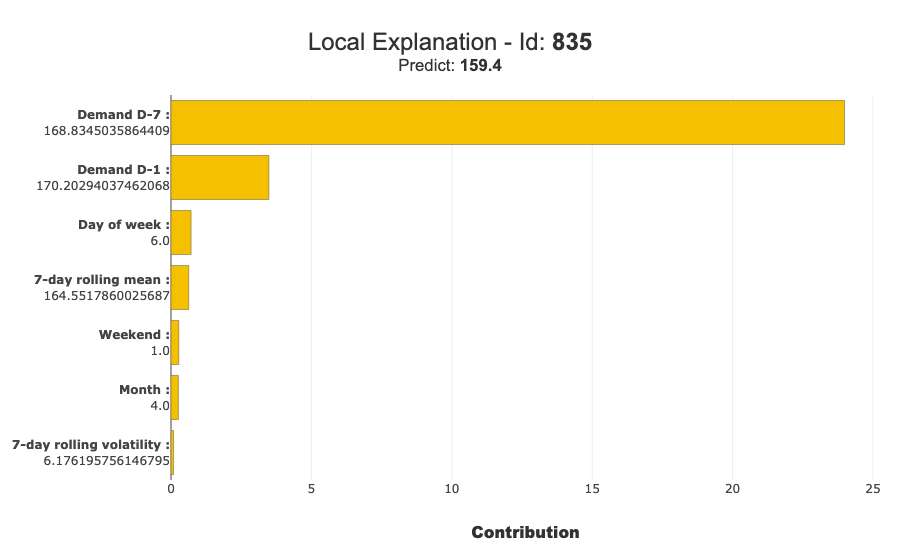
[7]:
worst_error_idx = (y_test.iloc[:, 0] - pred_test).abs().idxmax()
xpl.plot.local_plot(index=worst_error_idx)
5. Leakage checklist for temporal models
Use a strict time-based split (never random shuffling).
Compute rolling statistics using only past values.
Verify that calendar features are available at inference time.
Monitor drift in lag feature distributions in production.