Shapash Tutorial - NLP Explainability with TF-IDF Classification

This tutorial shows how to build a text classification model with TF-IDF + Logistic Regression and explain its predictions with Shapash.

You will learn how to: - prepare a simple NLP dataset, - train and evaluate a TF-IDF classifier, - inspect model behavior globally (important terms), - interpret a single prediction locally with Shapash.

import numpy as np
import pandas as pd

from sklearn.feature_extraction.text import TfidfVectorizer
from sklearn.linear_model import LogisticRegression
from sklearn.metrics import classification_report, accuracy_score
from sklearn.model_selection import train_test_split

from shapash import SmartExplainer

1. Build a small text classification dataset

We create a synthetic but realistic binary dataset: - satisfied: positive customer feedback - frustrated: negative customer feedback

We also add a subset of mitigated / mixed-sentiment messages (both pros and cons) to make some cases intentionally harder to classify.

rng = np.random.default_rng(42)

positive_templates = [
    "The product is {adj} and the support team was {support}.",
    "I had a {adj} experience, delivery was {delivery}.",
    "Everything worked {adv}, setup was {setup}.",
    "Great quality and {adj} customer care.",
]

negative_templates = [
    "The product is {adj} and support was {support}.",
    "I had a {adj} experience, delivery was {delivery}.",
    "Nothing worked {adv}, setup was {setup}.",
    "Poor quality and {adj} customer care.",
]

mitigated_templates = [
    "The product is {pos_adj} but delivery was {neg_delivery}.",
    "Support was {pos_support}, however setup felt {neg_setup}.",
    "The experience was {mix_adj}: quality was good, but service was {neg_support}.",
    "Delivery was {pos_delivery}, yet overall usage remained {neg_adj}.",
    "I can see value in it, although some steps were {neg_setup}.",
]

positive_words = {
    "adj": ["excellent", "great", "reliable", "smooth"],
    "support": ["helpful", "responsive", "professional"],
    "delivery": ["fast", "on time", "perfect"],
    "adv": ["perfectly", "very well", "flawlessly"],
    "setup": ["easy", "quick", "straightforward"],
}

negative_words = {
    "adj": ["bad", "awful", "unreliable", "frustrating"],
    "support": ["slow", "unhelpful", "absent"],
    "delivery": ["late", "delayed", "messy"],
    "adv": ["poorly", "badly", "inconsistently"],
    "setup": ["confusing", "hard", "broken"],
}

mitigated_words = {
    "pos_adj": ["useful", "promising", "decent"],
    "pos_support": ["kind", "available", "responsive"],
    "pos_delivery": ["on time", "acceptable", "fast"],
    "mix_adj": ["mixed", "acceptable", "inconsistent"],
    "neg_adj": ["frustrating", "rough", "unclear"],
    "neg_support": ["slow", "inconsistent", "hard to reach"],
    "neg_delivery": ["late", "unpredictable", "delayed"],
    "neg_setup": ["confusing", "hard", "not straightforward"],
}

label_map = {0: "frustrated", 1: "satisfied"}

def sample_sentence(template, vocab):
    return template.format(
        adj=rng.choice(vocab["adj"]),
        support=rng.choice(vocab["support"]),
        delivery=rng.choice(vocab["delivery"]),
        adv=rng.choice(vocab["adv"]),
        setup=rng.choice(vocab["setup"]),
    )

def sample_mitigated(template, vocab):
    return template.format(
        pos_adj=rng.choice(vocab["pos_adj"]),
        pos_support=rng.choice(vocab["pos_support"]),
        pos_delivery=rng.choice(vocab["pos_delivery"]),
        mix_adj=rng.choice(vocab["mix_adj"]),
        neg_adj=rng.choice(vocab["neg_adj"]),
        neg_support=rng.choice(vocab["neg_support"]),
        neg_delivery=rng.choice(vocab["neg_delivery"]),
        neg_setup=rng.choice(vocab["neg_setup"]),
    )

n_samples_per_class = 700
n_mitigated = 350
texts = []
labels = []
is_mitigated = []

for _ in range(n_samples_per_class):
    texts.append(sample_sentence(rng.choice(positive_templates), positive_words))
    labels.append(1)
    is_mitigated.append(0)

for _ in range(n_samples_per_class):
    texts.append(sample_sentence(rng.choice(negative_templates), negative_words))
    labels.append(0)
    is_mitigated.append(0)

# Add mixed-sentiment feedback with balanced labels to create harder boundary cases.
for i in range(n_mitigated):
    texts.append(sample_mitigated(rng.choice(mitigated_templates), mitigated_words))
    labels.append(1 if i < n_mitigated // 2 else 0)
    is_mitigated.append(1)

nlp_df = pd.DataFrame({"text": texts, "label": labels, "is_mitigated": is_mitigated})
nlp_df["label_name"] = nlp_df["label"].map(label_map)
nlp_df = nlp_df.sample(frac=1.0, random_state=42).reset_index(drop=True)
nlp_df.head()

	text	label	is_mitigated	label_name
0	Poor quality and frustrating customer care.	0	0	frustrated
1	Poor quality and awful customer care.	0	0	frustrated
2	I had a smooth experience, delivery was perfect.	1	0	satisfied
3	I had a awful experience, delivery was late.	0	0	frustrated
4	Support was available, however setup felt not ...	1	1	satisfied

2. Train a TF-IDF + Logistic Regression classifier

X_train_text, X_test_text, y_train, y_test = train_test_split(
    nlp_df["text"],
    nlp_df["label"],
    test_size=0.25,
    random_state=42,
    stratify=nlp_df["label"],
)

vectorizer = TfidfVectorizer(
    lowercase=True,
    ngram_range=(1, 2),
    min_df=2,
    max_features=800,
)

X_train_tfidf = vectorizer.fit_transform(X_train_text)
X_test_tfidf = vectorizer.transform(X_test_text)
feature_names = vectorizer.get_feature_names_out()

# Fit with named columns to avoid sklearn feature-name warnings downstream.
X_train_tfidf_df = pd.DataFrame(
    X_train_tfidf.toarray(),
    columns=feature_names,
    index=X_train_text.index,
)
X_test_tfidf_df = pd.DataFrame(
    X_test_tfidf.toarray(),
    columns=feature_names,
    index=X_test_text.index,
)

clf = LogisticRegression(max_iter=2000, random_state=42)
clf.fit(X_train_tfidf_df, y_train)

y_pred = clf.predict(X_test_tfidf_df)

print(f"Accuracy: {accuracy_score(y_test, y_pred):.3f}\n")
print("Classification report:\n")
print(
    classification_report(
        y_test,
        y_pred,
        labels=[0, 1],
        target_names=[label_map[0], label_map[1]],
    )
)

Accuracy: 0.900

Classification report:

              precision    recall  f1-score   support

  frustrated       0.86      0.95      0.90       219
   satisfied       0.94      0.85      0.89       219

    accuracy                           0.90       438
   macro avg       0.90      0.90      0.90       438
weighted avg       0.90      0.90      0.90       438

3. Quick global interpretability from logistic coefficients

Before Shapash, we can inspect the strongest positive/negative TF-IDF terms from the linear model coefficients.

feature_names = vectorizer.get_feature_names_out()
coef = clf.coef_[0]

coef_df = pd.DataFrame({"term": feature_names, "coef": coef}).sort_values("coef")

top_negative = coef_df.head(12).reset_index(drop=True)
top_positive = coef_df.tail(12).sort_values("coef", ascending=False).reset_index(drop=True)

print("Top terms pushing toward class:", label_map[clf.classes_[0]])
display(top_negative)
print("Top terms pushing toward class:", label_map[clf.classes_[1]])
display(top_positive)

Top terms pushing toward class: frustrated

	term	coef
0	poor quality	-2.291052
1	poor	-2.291052
2	bad	-2.025405
3	nothing worked	-2.022134
4	nothing	-2.022134
5	awful	-1.990413
6	and support	-1.983859
7	frustrating	-1.975218
8	unreliable	-1.946076
9	support was	-1.732814
10	was messy	-1.258450
11	messy	-1.258450

Top terms pushing toward class: satisfied

	term	coef
0	great	3.388834
1	great quality	2.243535
2	everything worked	2.027965
3	everything	2.027965
4	excellent	1.932006
5	smooth	1.884922
6	reliable	1.803459
7	team	1.480375
8	and the	1.480375
9	support team	1.480375
10	team was	1.480375
11	the support	1.480375

4. Explain predictions with Shapash

Shapash expects tabular inputs. For TF-IDF, each term is a feature, so we convert the sparse matrix into a DataFrame with term names as columns.

proba_values = pd.DataFrame(
    clf.predict_proba(X_test_tfidf_df)[:, 1],
    columns=[f"proba_{label_map[clf.classes_[1]]}"],
    index=X_test_tfidf_df.index,
)

predicted_code = pd.Series(
    clf.predict(X_test_tfidf_df),
    index=X_test_tfidf_df.index,
    name="predicted_code",
)
predicted_label = predicted_code.map(label_map).rename("predicted_label")

y_pred_numeric = predicted_code.astype(int).to_frame("y_pred")
y_target_numeric = y_test.astype(int).to_frame("y_target")

additional_data = pd.DataFrame({
    "raw_text": X_test_text,
    "is_mitigated": nlp_df.loc[X_test_text.index, "is_mitigated"],
    "true_label": y_test.map(label_map),
    "predicted_label": predicted_label,
})

xpl = SmartExplainer(
    model=clf,
    label_dict={0: "frustrated", 1: "satisfied"},
    title_story="TF-IDF NLP classification explainability",
)
xpl.compile(
    x=X_test_tfidf_df,
    y_pred=y_pred_numeric,
    y_target=y_target_numeric,
    additional_data=additional_data,
    columns_order=["raw_text",
                    "true_label",
                    "predicted_label",
                    ]+X_test_tfidf_df.columns.tolist()
)

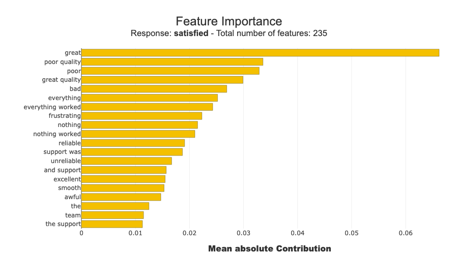
xpl.plot.features_importance(max_features=20)

INFO: Shap explainer type - shap.explainers.PermutationExplainer()

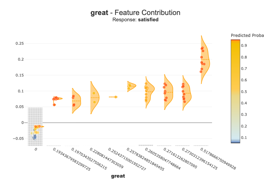
xpl.plot.contribution_plot(col=top_positive.loc[0, "term"])

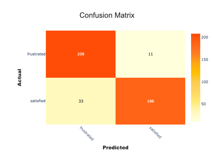
xpl.plot.confusion_matrix_plot()

# Prefer a misclassified example for a more insightful local explanation.
test_pred = predicted_code
misclassified_idx = y_test[y_test != test_pred].index

if len(misclassified_idx) > 0:
    sample_idx = misclassified_idx[0]
else:
    # Fallback: pick the closest probability to 0.5.
    confidence_gap = (proba_values.iloc[:, 0] - 0.5).abs()
    sample_idx = confidence_gap.idxmin()

print("Explained sample index:", sample_idx)
display(additional_data.loc[[sample_idx]])
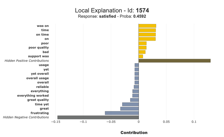
xpl.plot.local_plot(index=sample_idx)

Explained sample index: 1574

	raw_text	is_mitigated	true_label	predicted_label
1574	Delivery was on time, yet overall usage remain...	1	satisfied	frustrated

# Optional: launch the interactive Shapash webapp (uncomment to run).
app = xpl.run_app(title_story="TF-IDF NLP classification explainability", port=8060)

INFO:root:Your Shapash application run on http://PMP01087:8060/
INFO:root:Use the method .kill() to down your app.

5. Key takeaways

• TF-IDF + Logistic Regression is a strong and interpretable NLP baseline.

• Coefficients provide a first global view of influential terms.

• Shapash helps investigate both global and local prediction drivers in a unified interface.

Production tips

• Keep vectorizer and model versions aligned (same vocabulary at inference).

• Track vocabulary drift and out-of-vocabulary rate over time.

• Monitor class balance changes and confidence calibration.