
Shapash + TabICL for Regression
This tutorial shows how to: - train a TabICLRegressor on a regression problem - compute SHAP values with tabicl.shap - convert these contributions into a format compatible with Shapash - explore global and local explainability in a notebook - optionally launch the Shapash WebApp
The dataset used here is house_prices, already provided in Shapash.
1. Prerequisites
TabICL does not return Shapley values directly from predict(). However, the project does provide a tabicl.shap module that computes SHAP values by leveraging the native column-wise NaN masking.
Typical installation: pip install tabicl[shap]
On some macOS Intel environments, you may need to install PyTorch before tabicl.
[ ]:
# Uncomment if needed
# !pip install tabicl[shap]

import numpy as np
import pandas as pd
from sklearn.metrics import mean_absolute_error, mean_squared_error, r2_score
from sklearn.model_selection import train_test_split
from sklearn.preprocessing import OrdinalEncoder

from shapash import SmartExplainer
from shapash.data.data_loader import data_loading
from tabicl import TabICLRegressor
from tabicl.shap import get_shap_values, plot_shap
2. Load the Data
[2]:
house_df, house_dict = data_loading('house_prices')

y = house_df['SalePrice']
X = house_df.drop(columns=['SalePrice'])

X_train, X_test, y_train, y_test = train_test_split(
    X,
    y,
    train_size=0.75,
    random_state=42,
)

X_train.head()
[2]:
| MSSubClass | MSZoning | LotArea | Street | LotShape | LandContour | Utilities | LotConfig | LandSlope | Neighborhood | ... | OpenPorchSF | EnclosedPorch | 3SsnPorch | ScreenPorch | PoolArea | MiscVal | MoSold | YrSold | SaleType | SaleCondition | |
|---|---|---|---|---|---|---|---|---|---|---|---|---|---|---|---|---|---|---|---|---|---|
| Id | |||||||||||||||||||||
| 1024 | 1-Story PUD (Planned Unit Development) - 1946 ... | Residential Low Density | 3182 | Paved | Regular | Near Flat/Level | All public Utilities (E,G,W,& S) | Inside lot | Gentle slope | Bloomington Heights | ... | 20 | 0 | 0 | 0 | 0 | 0 | 5 | 2008 | Warranty Deed - Conventional | Normal Sale |
| 811 | 1-Story 1946 & Newer All Styles | Residential Low Density | 10140 | Paved | Regular | Near Flat/Level | All public Utilities (E,G,W,& S) | Inside lot | Gentle slope | Northwest Ames | ... | 0 | 0 | 0 | 0 | 648 | 0 | 1 | 2006 | Warranty Deed - Conventional | Normal Sale |
| 1385 | 1-1/2 Story Finished All Ages | Residential Low Density | 9060 | Paved | Regular | Near Flat/Level | All public Utilities (E,G,W,& S) | Inside lot | Gentle slope | Edwards | ... | 0 | 0 | 0 | 0 | 0 | 0 | 10 | 2009 | Warranty Deed - Conventional | Normal Sale |
| 627 | 1-Story 1946 & Newer All Styles | Residential Low Density | 12342 | Paved | Slightly irregular | Near Flat/Level | All public Utilities (E,G,W,& S) | Inside lot | Gentle slope | North Ames | ... | 0 | 36 | 0 | 0 | 0 | 600 | 8 | 2007 | Warranty Deed - Conventional | Normal Sale |
| 814 | 1-Story 1946 & Newer All Styles | Residential Low Density | 9750 | Paved | Regular | Near Flat/Level | All public Utilities (E,G,W,& S) | Inside lot | Gentle slope | North Ames | ... | 0 | 275 | 0 | 0 | 0 | 500 | 4 | 2007 | Court Officer Deed/Estate | Normal Sale |
5 rows × 72 columns
3. Train the TabICL Model
In this version, the data is encoded numerically before fit (ordinal encoding of categorical variables), and missing values are imputed before training.
The model is then trained on X_train_num and evaluated on X_test_num.
[3]:
# Replace missing values then encode categoricals to numeric before fit
num_cols = X_train.select_dtypes(include=['number', 'bool']).columns
cat_cols = X_train.columns.difference(num_cols)

X_train_filled = X_train.copy()
X_test_filled = X_test.copy()

num_fill_values = X_train_filled[num_cols].median()
X_train_filled[num_cols] = X_train_filled[num_cols].fillna(num_fill_values)
X_test_filled[num_cols] = X_test_filled[num_cols].fillna(num_fill_values)

if len(cat_cols) > 0:
    cat_fill_values = X_train_filled[cat_cols].mode(dropna=True).iloc[0]
    X_train_filled[cat_cols] = X_train_filled[cat_cols].fillna(cat_fill_values)
    X_test_filled[cat_cols] = X_test_filled[cat_cols].fillna(cat_fill_values)

    ordinal_encoder = OrdinalEncoder(
        handle_unknown='use_encoded_value',
        unknown_value=-1,
        encoded_missing_value=-1,
    )
    X_train_cat = pd.DataFrame(
        ordinal_encoder.fit_transform(X_train_filled[cat_cols]),
        index=X_train_filled.index,
        columns=cat_cols,
    )
    X_test_cat = pd.DataFrame(
        ordinal_encoder.transform(X_test_filled[cat_cols]),
        index=X_test_filled.index,
        columns=cat_cols,
    )
else:
    X_train_cat = pd.DataFrame(index=X_train_filled.index)
    X_test_cat = pd.DataFrame(index=X_test_filled.index)

X_train_num = pd.concat([X_train_filled[num_cols].astype(float), X_train_cat.astype(float)], axis=1)
X_test_num = pd.concat([X_test_filled[num_cols].astype(float), X_test_cat.astype(float)], axis=1)

# Keep the original feature order
X_train_num = X_train_num.reindex(columns=X_train.columns).fillna(0.0)
X_test_num = X_test_num.reindex(columns=X_train.columns).fillna(0.0)

regressor = TabICLRegressor(
    n_estimators=4,
    kv_cache=True,
    device='cpu',
    random_state=42,
)

regressor.fit(X_train_num, y_train)
[3]:
TabICLRegressor(device='cpu', kv_cache=True, n_estimators=4)In a Jupyter environment, please rerun this cell to show the HTML representation or trust the notebook.
On GitHub, the HTML representation is unable to render, please try loading this page with nbviewer.org.
Parameters
| n_estimators | 4 | |
| norm_methods | None | |
| feat_shuffle_method | 'latin' | |
| outlier_threshold | 4.0 | |
| batch_size | 8 | |
| kv_cache | True | |
| model_path | None | |
| allow_auto_download | True | |
| checkpoint_version | 'tabicl-regressor-v2-20260212.ckpt' | |
| device | 'cpu' | |
| use_amp | 'auto' | |
| use_fa3 | 'auto' | |
| offload_mode | 'auto' | |
| disk_offload_dir | None | |
| random_state | 42 | |
| n_jobs | None | |
| verbose | False | |
| inference_config | None |
[4]:
y_pred = pd.DataFrame(regressor.predict(X_test_num), columns=['pred'], index=X_test_num.index)

metrics = pd.Series({
    'MAE': mean_absolute_error(y_test, y_pred['pred']),
    'RMSE': np.sqrt(mean_squared_error(y_test, y_pred['pred'])),
    'R2': r2_score(y_test, y_pred['pred']),
})

metrics.round(4)
[4]:
MAE     13479.4658
RMSE    21565.9094
R2          0.9336
dtype: float64
4. Compute SHAP Values with TabICL
We only explain a subset of the test set to keep the notebook responsive.
[5]:
X_explain_columns = X_test_num.columns.tolist()

# X_explain = X_explain.fillna(0.0).astype(float)

shap_values = get_shap_values(
    estimator=regressor,
    X_test=X_test_num,
    attribute_names=X_explain_columns,
)

type(shap_values)
PermutationExplainer explainer: 366it [07:53, 1.32s/it]
[5]:
shap._explanation.Explanation
5. Convert to a Shapash-Compatible Format
Shapash accepts user-provided local contributions with SmartExplainer.compile(..., contributions=...). For regression, you simply provide an (n_samples, n_features) matrix aligned with x.
[6]:
contributions = pd.DataFrame(
    shap_values.values,
    columns=X_explain_columns,
    index=X_test_num.index,
)

contributions.head()
[6]:
| MSSubClass | MSZoning | LotArea | Street | LotShape | LandContour | Utilities | LotConfig | LandSlope | Neighborhood | ... | OpenPorchSF | EnclosedPorch | 3SsnPorch | ScreenPorch | PoolArea | MiscVal | MoSold | YrSold | SaleType | SaleCondition | |
|---|---|---|---|---|---|---|---|---|---|---|---|---|---|---|---|---|---|---|---|---|---|
| Id | |||||||||||||||||||||
| 893 | 1134.341146 | 1165.591146 | -4267.718750 | -243.335938 | -846.552083 | -1180.197917 | -129.291667 | -722.570312 | -959.122396 | -718.528646 | ... | -2731.927083 | -1290.799479 | -2229.411458 | 384.627604 | -3934.169271 | 324.828125 | -1374.604167 | -55.851562 | -1159.580729 | -3525.583333 |
| 1106 | 2210.226562 | 1919.864583 | 4093.882812 | -616.252604 | 54.406250 | -2897.070312 | -54.440104 | -442.393229 | -2222.575521 | 9676.208333 | ... | -975.208333 | -317.333333 | -2853.255208 | 580.546875 | -7612.604167 | 736.776042 | -1093.338542 | -518.557292 | -1599.414062 | -5408.106771 |
| 414 | -1800.076823 | -1522.001302 | -2821.118490 | -107.744792 | -535.144531 | -1283.110677 | -81.026042 | -792.263021 | -646.457031 | -2638.473958 | ... | -2467.863281 | 333.020833 | -2093.165365 | 191.466146 | -3519.006510 | 585.395833 | -988.803385 | -290.632812 | -970.368490 | -3135.895833 |
| 523 | 1554.544271 | -2411.419271 | -11190.130208 | -137.018229 | -1000.174479 | -2037.104167 | 172.817708 | 95.820312 | -1223.960938 | 4175.825521 | ... | -1240.661458 | -105.760417 | -2577.388021 | 366.585938 | -5503.609375 | 846.067708 | 301.609375 | -58.408854 | -1523.947917 | -4321.684896 |
| 1037 | 801.145833 | 1113.877604 | 4766.515625 | -670.895833 | -154.882812 | 3451.523438 | -229.979167 | -1795.559896 | -2748.388021 | 5653.872396 | ... | -2727.916667 | -969.276042 | -3819.666667 | 271.013021 | -9041.513021 | 94.385417 | 709.822917 | -470.518229 | -2645.000000 | -6211.145833 |
5 rows × 72 columns
6. Compile SmartExplainer with TabICL Outputs
[7]:
xpl = SmartExplainer(
    model=regressor,
    features_dict=house_dict,
    title_story='House Prices - TabICL Regressor',
)

xpl.compile(
    x=X_test_num,
    contributions=contributions,
    y_pred=y_pred,
    y_target=y_test,
)
7. Explainability in the Notebook
[8]:
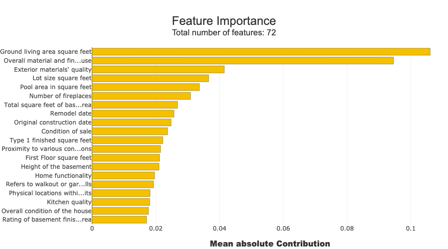
xpl.plot.features_importance()
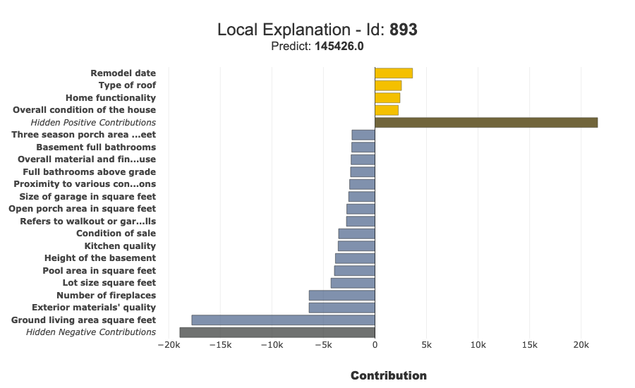
[9]:
example_index = X_test_num.index[0]
xpl.plot.local_plot(index=example_index)
[10]:
summary_df = xpl.to_pandas(max_contrib=4)
summary_df.head()
[10]:
| pred | feature_1 | value_1 | contribution_1 | feature_2 | value_2 | contribution_2 | feature_3 | value_3 | contribution_3 | feature_4 | value_4 | contribution_4 | |
|---|---|---|---|---|---|---|---|---|---|---|---|---|---|
| 893 | 145425.593750 | Ground living area square feet | 1068.0 | -17761.609375 | Exterior materials' quality | 0.0 | -6394.335938 | Number of fireplaces | 0.0 | -6384.5625 | Lot size square feet | 8414.0 | -4267.71875 |
| 1106 | 338848.625000 | Ground living area square feet | 2622.0 | 63718.979167 | Overall material and finish of the house | 8.0 | 30047.625 | Second floor square feet | 1122.0 | 10486.434896 | Number of fireplaces | 2.0 | 9939.911458 |
| 414 | 106041.742188 | Ground living area square feet | 1028.0 | -16405.161458 | Overall material and finish of the house | 5.0 | -11118.700521 | Proximity to various conditions | 2.0 | -10017.960938 | Exterior materials' quality | 0.0 | -5917.255208 |
| 523 | 157701.843750 | Lot size square feet | 5000.0 | -11190.130208 | Proximity to various conditions | 3.0 | -10930.195312 | Exterior materials' quality | 0.0 | -9621.018229 | Number of fireplaces | 2.0 | 9555.598958 |
| 1037 | 344184.750000 | Overall material and finish of the house | 9.0 | 62309.341146 | Original construction date | 2007.0 | 15426.658854 | Kitchen quality | 0.0 | 12653.299479 | Total square feet of basement area | 1620.0 | 12174.908854 |
8. Optionally Launch the WebApp
As in the other Shapash tutorials, you can launch the WebApp directly from the notebook.
[ ]:
app = xpl.run_app(port=8050)
# Then use: app.kill()
INFO:root:Your Shapash application run on http://PMP01087:8050/
INFO:root:Use the method .kill() to down your app.